Defining Properties

Scatter DLL Expert

TracePro Expert provides functionality to define phase functions for Bulk Scattering through compiled Dynamic Link Libraries (DLLs). Data from TracePro is passed into the DLL during raytrace. The DLL calculates a result, which is passed back to TracePro and used to scatter the ray. The Bulk Scatter Editor is used to select the desired DLL and to add user parameter data to control the calculations performed in the DLL. For more information about “User Defined Bulk Scatter”, see page 7.56.

Fluorescence Properties Expert

Fluorescence is modeled in TracePro through the use of a Fluorescence Property in combination with an object’s material properties. Fluorescence includes relative absorption and relative excitation normalized to the peak molar extinction coefficient, and relative emission. All of the values can be created with variation versus temperature and wavelength. Concentration of the fluorescing material can be set in the model by entering the molar concentration when applying the property to a solid object. A two stage ray trace is used when Fluorescence is enabled in the Raytrace Options. In the first stage of the ray trace, rays are traced in the excitation part of the material spectrum. A by-product of the first stage of the ray trace is that TracePro source files are generated which contain rays emanating from sites in the fluorescent material. The second stage of the ray trace uses the source files to trace fluorescent rays.

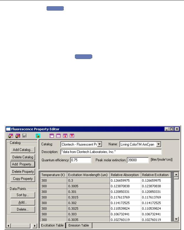
FIGURE 3.6 - Fluorescence Property Editor: Excitation Table

Fluorescence Properties

Defining Fluorescence Properties

Clicking on the Add Property button in the Catalog section of the Fluorescence Editor allows you to enter the data shown in the top tab of Figure 3.6:

•Descriptive text (optional)

•Quantum Efficiency

•Peak molar extinction

At this point, you can switch between entering excitation data (Figure 3.6) and emission data (Figure 3.7) by clicking on the appropriate tabs in the lower tab of the Fluorescence Property Editor.

Data to be entered in the Excitation Table:

•Temperature and Excitation Wavelength data - by clicking on the Add button in the Data Points section

•Relative Absorption during the excitation stage

•Relative Excitation during the excitation stage

FIGURE 3.7 - Fluorescence Property Editor: Emission Table

Data to be entered in the Emission Table:

•Temperature and Excitation Wavelength data - by clicking on the Add button in the Data Points section

•Relative Emission during the emission stage

The relative absorption, relative excitation, and relative emission values are normalized.

Defining Properties

Fluorescence Calculations

It is customary, in measuring fluorescence spectra, to express the peak molar extinction in base 10 rather than base e. The base 10 absorption coefficient is then

μa10(λ) = ab(λ)KpeakCmolar

where Kpeak is the peak molar extinction corresponding to the value of 1 in the

relative absorption ab(λ) , and Cmolar is the molar concentration in the particular sample. The transmittance through a sample of thickness t is then

–μ10t

τ = 10 a

The absorption coefficient used in a non-fluorescent material property in TracePro is related to the base 10 absorption coefficient by

μa = μa10 ln10

This is used for Lambert/Beer Law absorption, in which the transmittance through a thickness t is

τ = e–μat

The optics absorption coefficient µa is computed internally in TracePro for use by the raytrace. The same rule applies to the relative excitation values.

Note: the absorption coefficients: base 10, μa10 , or base e, μa ; and the

thickness, t, must be in the same units for these equations to be valid. For example if the first is in millimeters, the second should be in millimeters. However, note that the peak molar extinction, Kpeak, is in partial units of inverse

centimeters (see the first equation in this section and Figure 3.7. Though TracePro works by default in millimeters, the peak molar extinction is typically provided in partial units of inverse centimeters. Thus, as a suggestion to the user, it is best to remain consistent in the units of centimeters for these calculations.