Creating a Solid Model

the Default Model Rotations buttons, TracePro fills in the Rotation Angles for New Model entries according to the conventions outlined above. Use the To CAD button if the open model is in a CAD coordinate system and you are merging an optical design. Use the To Optics button if you have a lens design open and you are merging a CAD solid model. Optionally enter any coordinate shift between the two in the Translation for New Model fields. Finally, press Merge and the File Open dialog appears. Select the file you wish to merge and press OK.

Rotations are Euler rotations according to the right-hand rule. You can remember this using the mnemonic y-z-x. All rotations can be remembered using this rule, where the axes are always in the order x-y-z-x-y-z. Then an x rotation is y into z, and a z rotation is x into y.

Inserting Files

You can insert one model into another by using the Insert|Part menu item. You can keep files of standard parts on disk and insert them into existing models. Choosing the Insert|Part menu item opens the Open File dialog, but the model in the file is inserted into the currently open model instead of going into a new window.

Changing the Model View

TracePro allows you complete flexibility in changing the view of the model. You can have as many windows on each model open at one time as you wish. The view in each window is changed by using menu items on the View menu. Many of these are available on the View toolbar as well.

There are three types of views available in TracePro: Silhouette, Wireframe, Hidden Line and Render. Silhouette is the default view, the one that is active when you open TracePro or a new model. Wireframe view puts a wire grid on top of the surfaces to give a 3D impression of their shape. Render view makes the objects appear solid with shading based on the angle of incidence of an external, fictitious light source. The Render view assumes that the light source is located at the eye position of the viewer. All of the functions of TracePro can be carried out in any type of view. For example, you can select objects or Boolean operations in Silhouette, Render, Wireframe or Hidden Line view.

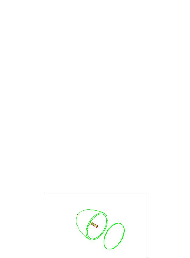
Figure 2.30 shows an example of a model viewed in Hiddenline mode.

FIGURE 2.30 - Hiddenline view of the Elliptical Reflector

Changing the Model View

The View|Set View dialog box shows the underlying philosophy behind setting the view in TracePro. This dialog box lets you set:

•Eye position

•Target Position

•Up Vector

•Perspective View On/Off

The eye position, target position and up vector can be set by entering numbers in this dialog box, or by manipulating the view interactively as described in the following sections.

The eye position is a point in 3D space from which the geometry is viewed. The target position is a point in 3D space that the eye is looking toward. When you set the target position, TracePro sets the current model window so that the target position is at the center of the window.

Sometimes the view may become clipped in TracePro, causing parts of the model to disappear or be cut off. This happens when the eye point is inside the model – parts of the model that are behind the eye point are not displayed. You can ameliorate this problem by changing the coordinates of the eye point so that they are outside the model using View|Set View, or by selecting View|Zoom All.

The Up vector is a vector in 3D space that determines the orientation of the view. When you set the up vector, TracePro rotates the view until the up vector lies in the plane of the screen pointing in the up direction.

The perspective check-box allows you to turn perspective viewing on or off to aid in visualizing the model.

Once you have entered the numbers you desire for controlling the view, press the Apply button to see the resulting view. However, you will probably find it more convenient to use the interactive viewing controls.

Silhouette Accuracy

In TracePro the model uses a facets to display objects and surfaces. In Silhouette mode you can use the View|High Resolution Silhouettes to improve the accuracy of the lines drawn in the Model Window. This mode is only available for Silhouettes and does require additional computational but the surfaces will be displayed at the proper positions for ray intersections.

Zooming

TracePro provides seven different ways of zooming the user’s window view in and out:

•Zoom In — Zooms in by a preset factor, the zoom factor is set in

View|Preferences

•Zoom Out — Zooms out by a preset factor, the zoom factor is set in

View|Preferences

•Zoom Ratio (no icon) — Opens a dialog box to type in a zoom factor

•Zoom Cursor — Zooms in as you hold down the left mouse button and move the mouse up in the TracePro model window, OR

—Zooms out as you hold down the left mouse button and move the mouse down in the TracePro model window, OR

Creating a Solid Model

if you have a wheel mouse, you can use the wheel to zoom in or zoom out, OR with a SHIFT-middle mouse button click.

•Zoom Window — Zooms to fit the rectangle formed by dragging a rubberband rectangle with the cursor. This can also be activated with a CTRL-middle mouse button click.

•Zoom All — Zooms in or out until all the objects in the model are visible in the window, with a margin of 10% around the edge.

•Zoom Selection — Zooms in or out until all the objects in current selection are visible in the window.

The preset factors for Zoom In and Zoom Out can be changed using the Zoom tab of the View|Preferences dialog box. The factory preset values are 2.0 and 0.5, respectively. A separate value, which is 1.1 by default, is used for the wheel mouse zooming.

Choosing Single-use zoom window means that after you complete a Zoom Window command, the Zoom Window mode is exited, and the toolbar button becomes unpressed. The default mode, in which the Single-use zoom window box is unchecked, means that Zoom Window remains in effect until you disable it by either clicking the Zoom Window toolbar button to toggle it, or by choosing another zoom or selection tool.

The Zoom In, Zoom Out, Zoom Window, Zoom Cursor, Zoom Selection, and Zoom All commands are available on the View toolbar.

Panning

The View|Pan menu item, also available on the View toolbar, allows you to move the view side to side and up and down. First choose the View|Pan menu item or press the Pan toolbar button to enter panning mode. Then, while holding down the mouse button, drag the mouse cursor around in the view. It is as though you are dragging the objects in the window, but you are really dragging the view. The Pan tool can be activated by pressing CTRL-right mouse button.

Panning is equivalent to moving the eye position and the target position in unison, keeping the target position in a plane perpendicular to the line between the two points.

Rotating the View

There are many different ways to rotate the view. They are accessed from two menu items:

•View|Profile

•View|Rotate

View|Profile lets you choose from five preset viewing angles: three orthogonal views and two oblique views. They can be chosen from the toolbar as well as the View|Profile menu. On the menu, the orthogonal views are listed as XY, XZ, and YZ, according to the axes that are visible in each view. The oblique or isometric views are illustrated by their buttons on the toolbar. The first, Iso 1, has the y-axis pointing up, the z-axis pointing to the right and toward you, and the x- axis to the right and away from you. The second, Iso 2, has the y-axis pointing up, the z-axis pointing to the right and away from you, and the x-axis to the left and