Examples

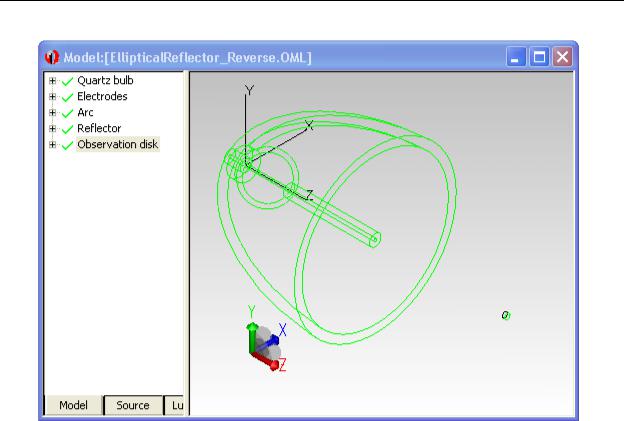
FIGURE 9.57 - EllipticalReflector_Reverse.oml example model from the TracePro examples directory. In a forward ray trace, rays are emitted from the Arc:Cyl surface source and flux collected at the Observation disk:Front surface. In a reverse ray trace, rays are emitted from the Observation Disk:Front surface and collected at the source.

In a reverse ray trace you can display all of these analysis results, but in some cases they have a different meaning. By way of going through this example, we will see how the meaning is different.

We will do a reverse ray trace in which rays are emitted from the Observation disk:Front surface. You can choose whatever surface you would like from which to start the reverse rays. The only requirement is that you first make the surface an exit surface.

Specifying reverse rays

Using the EllipticalReflector_Reverse.oml model, select the Observation disk:Front surface and then select Define|Apply Properties to open the Apply Properties dialog box. Select the Exit Surface tab, check the Exit surface checkbox, and enter 1000 for the Number of reverse rays, as shown in Figure 9.58. Click Apply to apply the setting to the surface.

Example Using Reverse Ray Tracing

FIGURE 9.58 - Apply Properties dialog box showing the exit surface defined. 1000 reverse rays have been applied to the exit surface.

Setting importance-sampling targets

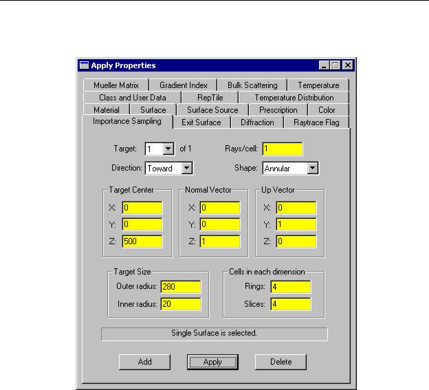
In order to make reverse ray tracing work, you must define importance-sampling targets for creating the reverse rays. The rays will be assigned an étendue value equal as described in the section “Theory of reverse ray tracing” on page 5.29, with solid angle determined by the importance-sampling target. Without one or more targets, the étendue cannot be calculated in a meaningful way. The target(s) are assigned to each exit surface from which reverse rays will be traced. In this example, we will use one importance sampling target and apply it to the Observation disk:Front surface. Select this surface and open the Apply Properties dialog box as in the previous section, but now select the Importance Sampling tab. We will create an annular importance sampling target at the front of the reflector, which is located at z = 500, with outer radius = 280 and inner radius = 20. We will also create cells on the importance-sampling target by dividing it into radial and azimuthal segments in a 4x4 pattern. Fill in the values shown in Figure 9.59 and click Apply to create the target. With these segments, for every reverse

Examples

ray specified, 4x4 = 16 rays will be generated. Because we specified 1000 reverse rays, 16,000 actual rays will be generated.

FIGURE 9.59 - Applying an importance sampling target to the Exit Surface.

Tracing Reverse Rays

Now we are ready to trace reverse rays. Select Raytrace|Reverse Raytrace to begin the ray trace. Alternatively, you can click the Reverse Trace button on the toolbar.

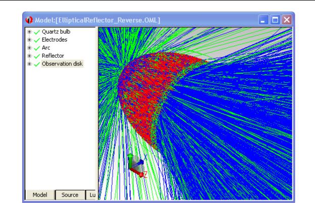
Once you start the ray-trace, the Audit progress dialog box will appear, followed by the Raytrace Progress dialog box, the same as for a forward ray trace. After the ray trace finishes, you are ready to view analysis results. Figure 9.60 shows the model window after the ray trace has finished, with rays displayed.

Example Using Reverse Ray Tracing

FIGURE 9.60 - Completed Reverse Ray-trace with rays displayed.

Viewing Analysis Results

Analysis results can be viewed in much the same way as for a forward ray trace, but sometimes the meaning is different. The differences and similarities are described in the sections below.

Irradiance/Illuminance Map

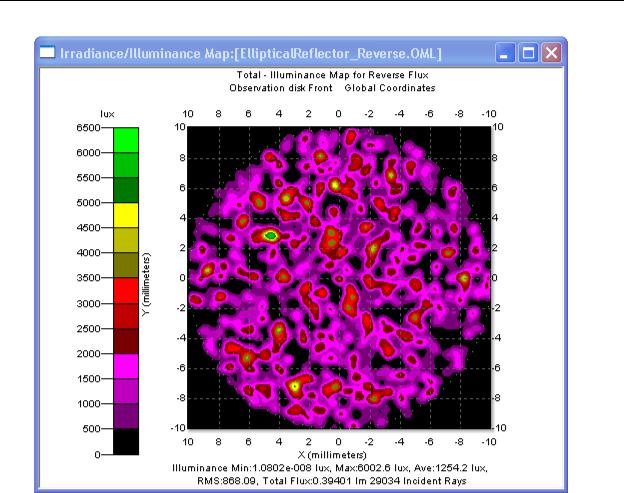
To display an irradiance/illuminance map at an exit surface, first select the exit surface and then select Analysis|Irradiance/Illuminance Maps, the same as you would for a forward ray trace. The incident illuminance on the exit surface will be displayed, the same as if the rays were traced forward. The Irradiance/ Illuminance map for our example is shown in Figure 9.61. Note that about 29,000 rays reached the observation disk. If you do a forward ray trace with 100,000 rays (this will take much longer than the reverse ray trace), only about 4,000 rays will reach the observation disk, resulting in a much noiser illuminance map.

Examples

FIGURE 9.61 - Illuminance map for reverse ray trace.

Example Using Reverse Ray Tracing

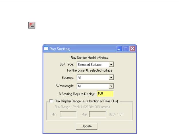
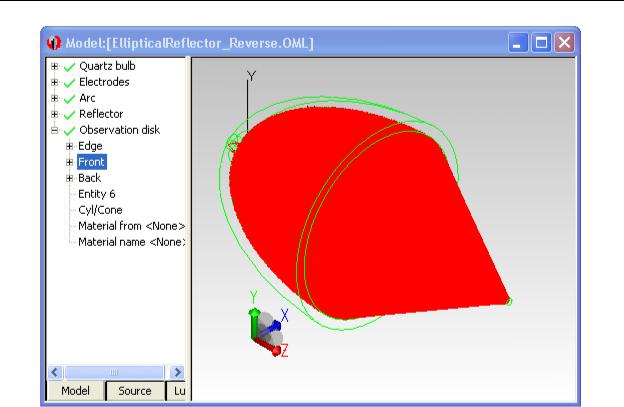
Ray Sorting

To show only the rays that produce irradiance/illuminance at the observation surface, select the Observation disk:Front surface and select Analysis|Ray Sorting. From the drop-down list, select Selected Surface as shown in Figure 9.62 and click Update. The only rays displayed are those that would have come from the source and struck the exit surface in a forward ray trace. The sorted rays are shown in Figure 9.63.

FIGURE 9.62 - Ray sorting dialog box with Sort Type set to Selected Surface.

Examples

FIGURE 9.63 - Sorted ray display with settings as shown in Figure 9.62.

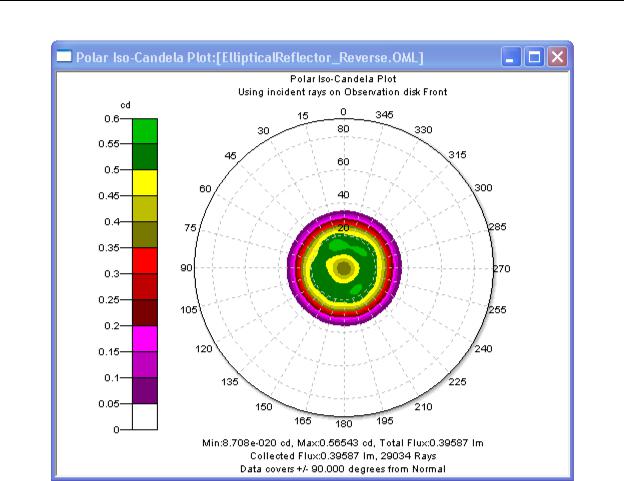
Candela Plot

The only options available for Candela plots are for rays incident on or exiting a surface, which you control via the Analysis|Candela Options dialog box. This is because in a reverse ray trace, rays always start from a surface, not from an infinite distance, as they would have to for a “missed rays” Candela plot. To view a polar iso-candela plot for rays incident on the Observation disk:Front surface, simply select the surface, then select Analysis|Candela Plots|Polar IsoCandela. The plot should appear as in Figure 9.64.

Example Using Reverse Ray Tracing

FIGURE 9.64 - Polar iso-candela plot for the Observation disk:Front surface.

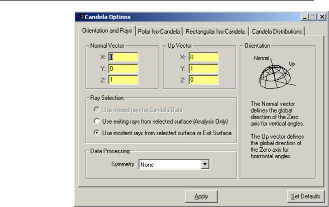
If the plot is blank or does not appear as in Figure 9.64, open the Analysis|Candela Options dialog box and check that the settings are as shown in Figure 9.65.

Examples

FIGURE 9.65 - Candela plot options to produce the plot in Figure 9.64. Note that the option Use missed rays for Candela Data is not available for a reverse ray trace.

If you select Use exiting rays from selected surface (Analysis Only) in the Candela Options dialog box and click Apply, the resulting plot will be blank. This is because the rays were started in reverse from the selected surface, so there are no rays exiting the surface in the forward direction.

The other candela plots are also available for a reverse ray trace. Refer to the TracePro User’s Manual for their use.

Example Using Reverse Ray Tracing

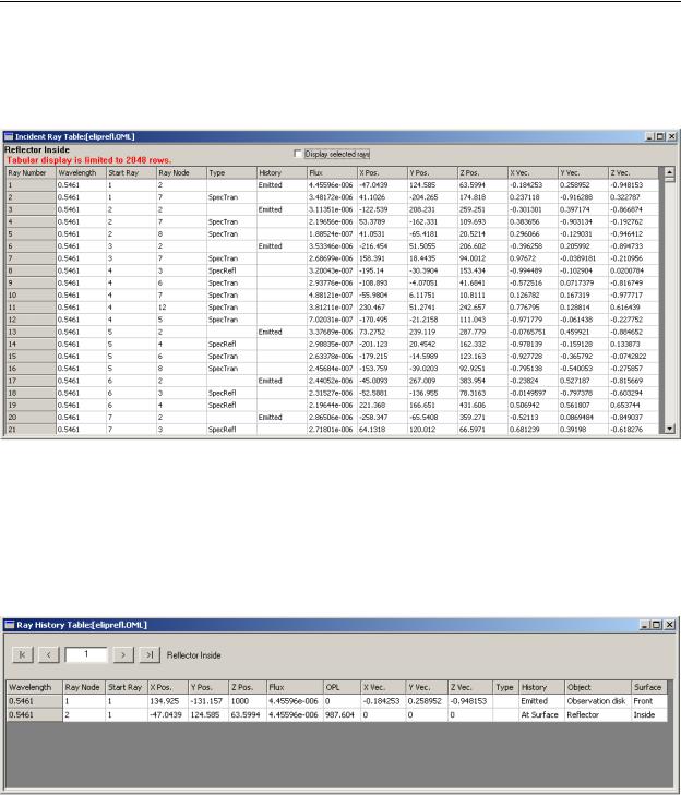
Incident Ray Table

The Incident Ray Table does not consider the sense of the rays, that is, it reports rays incident on the surface in the reverse direction. For example, select the

Reflector:Inside surface and then select Analysis|Incident Ray Table. The table will be displayed as shown in Figure 9.66.

FIGURE 9.66 - Example Incident Ray Table for the Reflector:Inside surface.

Ray History Table

The Ray History Table does not consider the sense of the rays, that is, it reports rays incident on the surface in the reverse direction. For example, select the Reflector:Inside surface and then select Analysis|Ray Histories. The table will be displayed as shown in Figure 9.67, with the history starting from the exit surface and proceeding to the reflector.

FIGURE 9.67 - Example Ray History Table for the Reflector:Inside surface.