
- •User’s Manual
- •COPYRIGHT
- •TRADEMARKS
- •LICENSE AGREEMENT
- •WARRANTY
- •DOCUMENT CONVENTIONS
- •What is TracePro?
- •Why Solid Modeling?
- •How Does TracePro Implement Solid Modeling?
- •Why Monte Carlo Ray Tracing?
- •The TracePro Graphical User Interface
- •Model Window
- •Multiple Models in Multiple Views
- •System Tree Window
- •System Tree Selection
- •Context Sensitive Menus
- •Model Window Popup Menus
- •System Tree Popup Menus
- •User Defaults
- •Objects and Surfaces
- •Changing the Names
- •Selecting Objects, Surfaces and Edges
- •Moving Objects and Other Manipulations
- •Interactive Viewing and Editing
- •Normal and Up Vectors
- •Modeling Properties
- •Applying Properties
- •Modeless Dialog Boxes
- •Expression Evaluator
- •Context Sensitive OnLine Help
- •Command Line Arguments
- •Increasing Access to RAM on 32-bit Operating Systems
- •Chinese Translations for TracePro Dialogs
- •Introduction to Solid Modeling
- •Model Units
- •Position and Rotation
- •Defining Primitive Solid Objects
- •Block
- •Cylinder/Cone
- •Torus
- •Sphere
- •Thin Sheet
- •Rubberband Primitives
- •Defining TracePro Solids
- •Lens Element
- •Lens tab
- •Aperture tab
- •Obstruction tab
- •Position tab
- •Aspheric tab
- •Fresnel Lens
- •Reflector
- •Conic
- •3D Compound
- •Parabolic Concentrators
- •Trough (Cylinder)
- •Compound Trough
- •Rectangular Concentrator
- •Facetted Rim Ray
- •Tube
- •Baffle Vane
- •Boolean Operations
- •Intersect
- •Subtract
- •Unite
- •Moving, Rotating, and Scaling Objects
- •Translate
- •Move
- •Rotate
- •Scale
- •Orientation
- •Sweeping and Revolving Surfaces
- •Sweep
- •Revolve
- •Notes Editor
- •Importing and Exporting Files
- •Exchanging Files with Other ACIS-based Software
- •Importing an ACIS File
- •Exporting an ACIS File
- •Stereo Lithography (*.STL) Files
- •Additional CAD Translators (Option)
- •Plot formats for model files
- •Healing Imported Data
- •How to Autoheal an Object
- •How to Manually Heal an Object
- •Reverse Surfaces (and Surface Normal)
- •Combine
- •Lens Design Files
- •Merging Files
- •Inserting Files
- •Changing the Model View
- •Silhouette Accuracy
- •Zooming
- •Panning
- •Rotating the View
- •Named Views
- •Previous View
- •Controlling the Appearance of Objects
- •Display Object
- •Display All
- •Display Object WCS
- •Display RepTile
- •Display Importance
- •Customize and Preferences
- •Preferences
- •Customize
- •Changing Colors
- •Overview
- •What is a property?
- •Define or Apply Properties
- •Property Editors
- •Toolbars and Menus
- •Command Panel
- •Information Panel
- •Grid Panel
- •Material Properties
- •Material Catalogs
- •Material Property Database
- •Create a new material property
- •Editing an existing material property
- •Exporting a material property
- •Importing a Material Property
- •Bulk Absorption
- •Birefringence
- •Bulk Scatter Properties
- •Bulk Scatter Property Editor
- •Import/Export
- •Scatter DLL
- •Fluorescence Properties
- •Defining Fluorescence Properties
- •Fluorescence Calculations
- •Fluorescence Ray Trace
- •Raytrace Options
- •Surface Source Properties
- •Surface Source Property Editor
- •Create a New Surface Source Property
- •Edit an Existing Surface Source Property
- •Export a Surface Source Property
- •Import a Surface Source Property
- •Gradient Index Properties
- •Gradient Index Property Editor
- •Create a New Gradient Index Property
- •Edit an Existing Gradient Index Property
- •Export a Gradient Index Property
- •Import a Gradient Index Property
- •Surface Properties
- •Using the Surface Property Database
- •Using the Surface Property Editor
- •Using Solve for
- •Direction-Sensitive Properties
- •Creating a new surface property
- •Editing an Existing Surface Property
- •Exporting a Surface Property
- •Importing a Surface Property
- •Surface Property Plot Tab
- •Incident Medium
- •Substrate Medium
- •by angle (deg)
- •by wavelength (um)
- •Display Values
- •Table BSDF
- •Creating a Table BSDF Property
- •Creating an Asymmetric Table BSDF Property
- •Using an Asymmetric Table BSDF property
- •Wire Grid Polarizers
- •Upgrading an older property database
- •Applying Wire-Grid Surface Properties
- •Thin Film Stacks
- •Using the Stack Editor
- •Thin Film Stack Editing Note
- •Entering a Single Layer Stack
- •RepTile Surfaces
- •Overview
- •Specifying a RepTile surface
- •RepTile Shapes
- •RepTile Geometries
- •RepTile Parameterization
- •Variables
- •Parameterized Input Fields
- •Decentering RepTile Geometry
- •Property Database Tools
- •Import
- •Export
- •Using Properties
- •Limitations in Pre-Defined Property Data
- •Applying Property Data
- •Material Properties
- •Material Catalogs
- •Applying Material Properties
- •Applying Birefringent Material Properties
- •Bulk Scattering
- •Fluorescence Properties
- •Applying Fluorescence Properties
- •Gradient Index Properties
- •Surface Properties
- •Using the Surface Property Database
- •Surface Source Properties
- •Blackbody Surface Sources
- •Blackbody and Graybody Calculations
- •Source Spreadsheet
- •Scaling the Total Rays for Several Sources
- •Prescription
- •Color
- •Importance Sampling
- •Defining Importance Sampling Targets (Manually)
- •Adding Targets
- •Number of Importance Rays
- •Shape, Dimensions, and Location of Importance Targets
- •Cells
- •Apply the Importance Sampling Property
- •Automatic Setup of Importance Sampling
- •Define the Prescription
- •Select the Target Shape
- •Apply, Cancel, or Save Targets
- •Editing/Deleting Importance Sampling Targets
- •Exit Surface
- •Predefined irradiance map orientation
- •Diffraction
- •Defining Diffraction in TracePro
- •Do I need to Model Diffraction in TracePro?
- •How do I Set Up Diffraction?
- •Using the Raytrace Flag
- •Mueller Matrix
- •Temperature
- •Class and User Data
- •RepTile Surfaces
- •Overview
- •Specifying a RepTile surface
- •Boundary Shapes
- •Export
- •Visualization and Surface Properties
- •Specifying a RepTile Texture File Surface
- •Bump Designation for Textured RepTile
- •Base Plane Designation for Textured RepTile
- •Temperature Distribution
- •Introduction to Ray Tracing
- •Combining Sources
- •Managing Sources with the System Tree
- •Managing Sources with the Source/Wavelength Selector
- •Defining Sources
- •Grid Sources
- •Setting Up the Grid
- •Grid Density: Points/Rings
- •Beam Setup
- •Wavelengths
- •Polarization
- •Surface Sources
- •Importance Sampling from Surface Sources
- •File Sources
- •Creating a File Source from Radiant Imaging Data
- •Creating a File Source from an Incident Ray Table
- •Creating a File Source from Theoretical or Measured Data
- •Insert Source
- •Capability to “trace every nth ray”
- •Capability to scale flux
- •Modify the File Source
- •Orienting and Selecting Sources
- •Multi-Selecting Sources
- •Move and Rotate Dialogs
- •Tracing Rays
- •Standard (Forward) Raytrace
- •Reverse Ray Tracing
- •Specifying reverse rays
- •Theory of reverse ray tracing
- •Luminance/Radiance Ray Tracing
- •Raytrace Options
- •Options
- •Analysis Units
- •Ray Splitting
- •Specular Rays Only
- •Importance Sampling
- •Aperture Diffraction and Aperture Diffraction Distance
- •Random Rays
- •Fluorescence
- •Polarization
- •Detect Ray Starting in Bodies
- •Random Seed
- •Wavelengths
- •Thresholds
- •Simulation and Output
- •Collect Exit Surface Data
- •Collect Candela Data
- •Index file name
- •Save Data to Disk during Raytrace
- •Save Ray History to disk
- •Sort Ray Paths
- •Save Bulk Scatter data to disk
- •Simulation Options for TracePro LC
- •Collect Exit Surface Data
- •Collect Candela Data
- •Advanced Options
- •Voxelization Type
- •Voxel Parameters
- •Raytrace Type
- •Gradient Index Substep Tolerance
- •Maximum Nested Objects
- •Progress Dialog
- •Ray Tracing modes
- •Analysis Mode
- •Saving and Restoring a Ray-Trace
- •Simulation Mode
- •Simulation Dialog
- •Simulation Options
- •Simulation Data for LC
- •Examining Raytrace Results
- •Analysis Menu
- •Display Rays
- •Ray Drawing Options
- •Ray Colors
- •Flux-based ray colors
- •Wavelength-based ray colors
- •Source-based ray colors
- •All rays one color
- •Irradiance Maps
- •Irradiance Map Options
- •Map Data
- •Display Options
- •Contour Levels
- •Access to Irradiance Data
- •Ensquared Flux
- •Luminance/Radiance Maps
- •3D Irradiance Plot
- •Candela Plots
- •Candela Options
- •Orientation and Rays
- •Polar Iso-Candela
- •Rectangular Iso-Candela
- •Candela Distributions
- •IESNA and Eulumdat formats
- •Access to Candela/Intensity Data
- •Enclosed Flux
- •Polarization Maps
- •Polarization Options
- •Save Polarization Data
- •OPL/Time-of-flight plot
- •OPL/Time-of-flight plot options
- •Incident Ray Table
- •Copying and Pasting the Incident Ray Table Data
- •Saving the Incident Ray Table in a File
- •Saving the Incident Ray Table as a Source File
- •Display Selected Rays
- •Source Files - Binary file format
- •Ray Histories
- •Copying and Pasting the Ray History Table Data
- •Saving the Ray History Table in a File
- •Ray Sorting
- •Ray Sorting Examples
- •Reports Menu
- •Flux Report
- •Property Data Report
- •Raytrace Report
- •Saving and Restoring a Raytrace
- •Tools Menu
- •Audit
- •Delete Raydata Memory
- •Collect Volume Flux
- •Overview
- •View Volume Flux
- •Overview
- •Flux Type
- •Normal Axis/Orientation
- •Slices
- •Color Map
- •Gradient
- •Logarithmic
- •Simulation File Manager
- •Irradiance/Illuminance Viewer
- •Overview
- •Viewing a saved Irradiance/Illuminance Map
- •Irradiance/Illuminance Viewer Options
- •Adding and Subtracting Irradiance/Illuminance Maps
- •Measurement Dialog
- •Introduction
- •The Use of Ray Splitting in Monte Carlo Simulation
- •Importance Sampling
- •Importance Sampling and Random Rays
- •When Do I Need Importance Sampling?
- •How to Choose Importance Sampling Targets
- •Importance Sampling Example
- •Material Properties
- •Material Property Database
- •Material Property Interpolation
- •Gradient Index Profile Polynomials
- •Complex Index of Refraction
- •Surface Properties
- •Coincident Surfaces
- •BSDF
- •Harvey-Shack BSDF
- •ABg BSDF Model
- •BRDF, BTDF, and TS
- •Elliptical BSDF
- •What is an elliptical BSDF?
- •Elliptical ABg BSDF model
- •Elliptical Gaussian BSDF
- •Calculation of Fresnel coefficients during raytrace
- •Anisotropic Surface Properties
- •Anisotropic surface types
- •Getting anisotropic data
- •User Defined Surface Properties
- •Overview
- •Creating a Surface Property DLL
- •Create the Surface Property
- •Apply Surface Property
- •API Specification for Enhanced Coating DLL
- •Document Layout
- •Calling Frequencies
- •Return Codes, Signals, and Constants -- TraceProDLL.h
- •Description of Return Codes
- •Function: fnInitDll
- •Function: fnEvaluateCoating
- •Function: fnAnnounceOMLPath
- •Function: fnAnnounceDataDirectory
- •Function: fnAnnounceSurfaceInfo
- •Function: fnAnnounceLocalBoundingBox
- •Function: fnAnnounceRaytraceStart
- •Function: fnAnnounceWavelengthStart
- •Function: fnAnnounceWavelengthFinish
- •Function: fnAnnounceRaytraceFinish
- •Example of Enhanced Coating DLL
- •Surface Source Properties
- •Spectral types
- •Rectangular
- •Gaussian
- •Solar
- •Table
- •Angular Types
- •Lambertian
- •Uniform
- •Gaussian
- •Solar
- •Table
- •Mueller Matrices and Stokes Vectors
- •Bulk Scattering
- •Henyey-Greenstein Phase Function
- •Gegenbauer Phase Function
- •Scattering Coefficient
- •Using Bulk Scattering in TracePro
- •User Defined Bulk Scatter
- •Using Scatter DLLs
- •Required DLL Functions called from TracePro
- •Common Arguments passed from TracePro
- •DLL Export Definitions
- •Non-Uniform Temperature Distributions
- •Overview
- •Distribution Types
- •Rectangular Coordinates
- •Circular Coordinates
- •Cylindrical Coordinates
- •Defining Temperature Distributions
- •Format for Temperature Distribution Storage Files
- •Type 0: Rectangular with Interpolated Points
- •Type 1: Rectangular with Polynomial Distribution
- •Type 2: Circular with Interpolated Points
- •Type 3: Circular with Polynomial Distribution
- •Type 4: Cylinder with Interpolated Points
- •Type 5: Cylinder with Polynomial Distribution
- •Polynomial Approximations of Temperature Distributions
- •Interpretation of Polar Iso-Candela Plots
- •Property Import/Export Formats
- •Material Property Format
- •Surface Property Format
- •Surface Data Columns
- •Grating Data Columns
- •Stack Property Format
- •Gradient Index Property Format
- •Gradient Index Data Columns (non-GRADIUM types)
- •Gradient Index Data Columns (GRADIUM (Buchdahl) type)
- •Gradient Index Data Columns (GRADIUM (Sellmeier) type)
- •Bulk Scatter Property Format
- •Fluorescence Property Format
- •Surface Source Property Format
- •RepTile Property Format
- •Texture File Format
- •The Scheme Language
- •Scheme Editor
- •Overview
- •Text Color
- •Macro Recorder
- •Recording States
- •Macro Format and Example
- •Macro Command Examples
- •Running a Macro Command from the Command Line
- •Running a Scheme Program Stored in a File
- •Scheme Commands
- •Creating Solids
- •Create a solid block:
- •Create a solid block named blk1:
- •Create a solid cylinder:
- •Create a solid elliptical cylinder:
- •Create a solid cone:
- •Create a solid elliptical cone:
- •Create a solid torus:
- •Boolean Operations
- •Boolean subtract
- •Boolean unite
- •Boolean intersect
- •Chamfers and blends
- •Macro Programs
- •Accessing TracePro Menu Selections using Scheme
- •For more information on Scheme
- •TracePro DDE Interface
- •Introduction
- •The Service Name
- •The Topic
- •The Item
- •Clipboard Formats
- •TracePro DDE Server
- •Establishing a Conversation
- •Excel 97/2000 Example
- •RepTile Examples
- •Fresnel lens
- •Conical hole geometry with variable geometry, rectangular tiles and rectangular boundary
- •Parameterized spherical bump geometry with staggered ring tiles
- •Aperture Diffraction Example
- •Applying Importance Sampling to a Diffracting Surface
- •Volume Flux Calculations Example
- •Sweep Surface Example
- •Revolve Surface Example
- •Using Copy with Move/Rotate
- •Example of Orienting and Selecting Sources
- •Creating the TracePro Source Example OML
- •Moving and Rotating the Sources from the Example
- •Anisotropic Surface Property
- •Creating an anisotropic surface property in TracePro
- •Applying an anisotropic surface property to a surface
- •Elliptical BSDF
- •Creating an Elliptical BSDF property
- •Applying an elliptical BSDF surface property to a surface
- •Using TracePro Diffraction Gratings
- •Using Diffraction Gratings in TracePro
- •Ray-tracing a Grating Surface Property
- •Example Using Reverse Ray Tracing
- •Specifying reverse rays
- •Setting importance-sampling targets
- •Tracing Reverse Rays
- •Viewing Analysis Results
- •Example using multiple exit surfaces
- •Example Using Luminance/Radiance Maps
- •Index

Creating a Solid Model
Lens Element
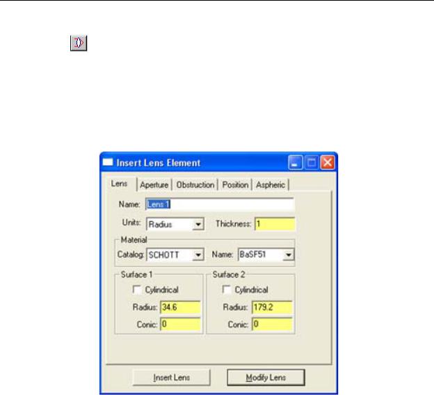
The Insert|Lens Element menu or Insert Lens toolbar button opens a tabbed dialog box that allows you to specify completely a lens element including curvatures (or radii); thickness; material; aperture and obstruction shape and dimensions; and position and orientation of the element. You can make a mirror using Insert|Lens Element by creating the mirror with the desired shape, then applying a reflective coating to it.
Note: An obstruction is a common term from lens design. An obstruction in TracePro creates a hole in the lens.
FIGURE 2.8 - Insert Lens Element dialog box: Lens tab
After you have entered all the data to specify the element press Insert Lens at the bottom of the dialog box to create the element. You can create as many elements as you wish. Simply edit the data for the new element and press Insert Lens again. To close the dialog box, click on the close button on the top bar of the dialog box, or press the Esc Key on your keyboard.
The Insert|Lens Element dialog box is a modeless dialog box, so you can leave it open while you do other things like inserting other solid objects, moving objects, changing the view, or applying properties.
Note the Modify Lens button in Figure 2.8. You can select an existing Lens object and then use the Insert|Lens Element dialog box to access and change the data by pressing the Modify Lens button. Note that the Modify button will be disabled if you don’t have an appropriate Lens selected in the model window.
An example of inserting a lens developed in the OSLO lens design software is shown in “Anisotropic Surface Property” on page 9.45
2.8 |
TracePro 5.0 User’s Manual |

Defining TracePro Solids
Lens tab
Using the lens tab you can enter
1.Curvature or Radius of each surface
2.Conic constant of each surface
3.Center thickness, the vertex to vertex between the two surfaces.
4.Material Catalog
5.Material Name
If you check one of the Cylindrical boxes, the dialog will change the conic constant to rotation. The rotation entry specifies the angle about the z-axis to rotate the cylinder in degrees.
The default glass is SCHOTT BK7.
Once you have completely specified the lens, press Insert Lens, and the lens will be created. The surfaces are created according to the sag equation
c |
ν |
ρ2 |
|
+ ∑Aι ρι, |
|
z= |
|
|
(2.1) |
||
|
2 |
2 |
|||
1 + 1 – (1 + K)c v ρ |
|
ι = 1 |
|
where ρ2=X2+Y2, cν is the curvature of the surface, K is the conic constant and Ai
is an aspheric coefficient. The X, Y, Z coordinates above are local coordinates relative to the vertex of the surface. See “Aspheric tab” on page 2.12 for details on entering Aspheric lens terms.
TABLE 2.1. Conic Constant Values
K (Conic Constant) |
Conic Type |
|
|
less than -1 |
hyperboloid |
|
|
-1 |
paraboloid |
|
|
between -1 and 0 |
ellipsoid |
|
|
0 |
spheroid |
|
|
greater than 0 |
oblate spheroid |
|
|
To edit a lens element, as a general rule select the Modify button in the Insert|Lens Element dialog box (version 1.4 files or later). The Modify button lets you make a series of sequential edits.
Here are the steps to alter a lens element:
1.Select the lens object in the model window or on the system tree.
2.Select Insert|Lens Element.
3.Edit the data and click Modify Lens in the dialog box.
TracePro applies your changes.
If you use another tool to edit a lens element—selecting one of the Boolean operations, for example—TracePro no longer recognizes that the lens element is still a “lens element.” For example, if you subtract a cylinder from a lens by the means of a Boolean operation, TracePro sees the result as a generic object rather than a lens object. Of course you can use the “obstruction” tabbed dialog to
TracePro 5.0 User’s Manual |
2.9 |

Creating a Solid Model
accomplish the same step as long as the cylinder is aligned along the axis of the lens, but in this case the lens object status is retained.
In general, altering a lens element is best done by selecting Modify Lens from the Insert|Lens Element dialog box. Editing the lens element in this way lets you go back as often as you want to make further changes.
Aperture tab
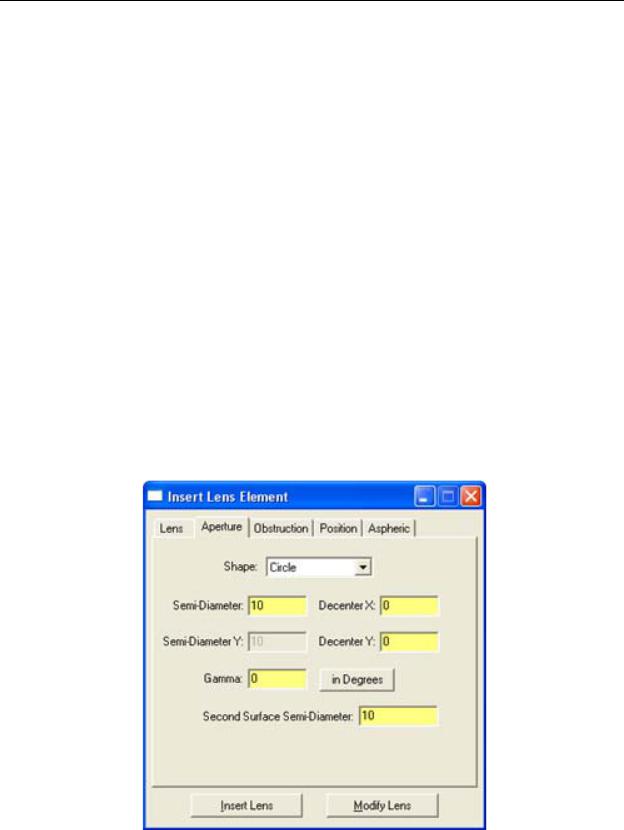
Using the Aperture tab (see Figure 2.9) you set:
1.Aperture shape: defines the cross-sectional shape of the lens orthogonal to the axis. It can be Circle, Rectangle, or Ellipse;
2.Aperture semi-diameter:s the radii of the lens aperture in the X and Y directions in the model units. Note that the Y dimension is not allowed for a circle shape;
3.Aperture Decenters: the decenter of the lens in the X and Y directions in the model units;
4.Aperture gamma: the orientation of the lens with respect to the optical axis, with X denoting the local horizontal axis and Y the local vertical axis. The value, either in Degrees or in Radians denotes the rotation of the lens around the local Z (i.e., optical) axis; and
5.Aperture second surface semi-diameter: allows for the second surface of a single lens to have a different semi-diameter than that of the first surface. Prescriptions from lens design codes (e.g., OSLO) often have this situation; therefore, the inclusion of this additional parameter ensures there is no spurious loss of aperture data when clicking on the Modify Lens button
FIGURE 2.9 - Insert Lens Element dialog box: Aperture tab
2.10 |
TracePro 5.0 User’s Manual |

Defining TracePro Solids
Obstruction tab
The obstruction used by TracePro refers to an opening or hole in the lens. To truly obscure a portion of the lens, insert a thin block or cylinder with an opaque Surface Property. Using the Obstruction tab (see Figure 2.10)you set:
1.Obstruction shape: options are None, Circle, Rectangle, and Ellipse;
2.Obstruction semi-diameters: the radii of the obstruction in the local X and Y directions in the model units;
3.Obstruction decenters: the decenters from the local optical axis of the obstruction in the local X an Y directions in the model units; and
4.Obstruction gamma: the orientation of the obstruction with respect to the optical axis, with X denoting the local horizontal axis and Y the local vertical axis. The value, either in Degrees or in Radians denotes the rotation of the obstruction around the local Z (i.e., optical) axis
The obstruction shape options are none, circle, rectangle, or ellipse.
FIGURE 2.10 - Insert Lens Element dialog box: Obstruction tab
Position tab
Using the Position tab (see Figure 2.11) you set:
1.The X, Y, Z coordinates of the vertex of the first surface of the element, in global coordinates;
2.The X, Y, Z rotation angles (tilt) of the first surface or entire element;
3.The X, Y, Z decenters of the second surface with respect to the first suface (i.e., these are local offsets with respect to item (1) above); and
TracePro 5.0 User’s Manual |
2.11 |