ЦОС_Заочники2013 / Книги по ЦОС / Дополнительная литература / Основы ЦОС (на англ.яз) / MS5

FAST FOURIER TRANSFORMS

SECTION 5

FAST FOURIER TRANSFORMS

■The Discrete Fourier Transform

■The Fast Fourier Transform

■FFT Hardware Implementation and Benchmarks

■DSP Requirements for Real Time FFT Applications

■Spectral Leakage and Windowing

5.a

FAST FOURIER TRANSFORMS

5.b

FAST FOURIER TRANSFORMS

SECTION 5

FAST FOURIER TRANSFORMS

Walt Kester

THE DISCRETE FOURIER TRANSFORM

In 1807 the French mathematician and physicist Jean Baptiste Joseph Fourier presented a paper to the Institut de France on the use of sinusoids to represent temperature distributions. The paper made the controversial claim that any continuous periodic signal could be represented by the sum of properly chosen sinusoidal waves. Among the publication review committee were two famous mathematicians: Joseph Louis Lagrange, and Pierre Simon de Laplace. Lagrange objected strongly to publication on the basis that Fourier’s approach would not work with signals having discontinuous slopes, such as square waves. Fourier’s work was rejected, primarily because of Lagrange’s objection, and was not published until the death of Lagrange, some 15 years later. In the meantime, Fourier’s time was occupied with political activities, expeditions to Egypt with Napoleon, and trying to avoid the guillotine after the French Revolution! (This bit of history extracted from Reference 1, p.141).

It turns out that both Fourier and Lagrange were at least partially correct. Lagrange was correct that a summation of sinusoids cannot exactly form a signal with a corner. However, you can get very close if enough sinusoids are used. (This is described by the Gibbs effect, and is well understood by scientists, engineers, and mathematicians today).

Fourier analysis forms the basis for much of digital signal processing. Simply stated, the Fourier transform (there are actually several members of this family) allows a time domain signal to be converted into its equivalent representation in the frequency domain. Conversely, if the frequency response of a signal is known, the inverse Fourier transform allows the corresponding time domain signal to be determined.

In addition to frequency analysis, these transforms are useful in filter design, since the frequency response of a filter can be obtained by taking the Fourier transform of its impulse response. Conversely, if the frequency response is specified, then the required impulse response can be obtained by taking the inverse Fourier transform of the frequency response. Digital filters can be constructed based on their impulse response, because the coefficients of an FIR filter and its impulse response are identical.

The Fourier transform family (Fourier Transform, Fourier Series, Discrete Time Fourier Series, and Discrete Fourier Transform) is shown in Figure 5.2. These accepted definitions have evolved (not necessarily logically) over the years and depend upon whether the signal is continuous–aperiodic, continuous–periodic, sampled–aperiodic, or sampled–periodic. In this context, the term sampled is the same as discrete (i.e., a discrete number of time samples).

5.1

FAST FOURIER TRANSFORMS

APPLICATIONS OF THE DISCRETE

FOURIER TRANSFORM (DFT)

Digital Spectral Analysis

Spectrum Analyzers

Speech Processing

Imaging

Pattern Recognition

Filter Design

Calculating Impulse Response from Frequency Response

Calculating Frequency Response from Impulse Response

The Fast Fourier Transform (FFT) is Simply an Algorithm for Efficiently Calculating the DFT

Figure 5.1

FOURIER TRANSFORM FAMILY

AS A FUNCTION OF TIME DOMAIN SIGNAL TYPE

FOURIER TRANSFORM: Signal is Continuous and Aperiodic

t

FOURIER SERIES: Signal is Continuous and Periodic

t

DISCRETE TIME FOURIER SERIES: Signal is Sampled and Aperiodic

Figure 5.2

5.2

FAST FOURIER TRANSFORMS

The only member of this family which is relevant to digital signal processing is the

Discrete Fourier Transform (DFT) which operates on a sampled time domain signal which is periodic. The signal must be periodic in order to be decomposed into the summation of sinusoids. However, only a finite number of samples (N) are available for inputting into the DFT. This dilemma is overcome by placing an infinite number of groups of the same N samples “end-to-end,” thereby forcing mathematical (but not real-world) periodicity as shown in Figure 5.2.

The fundamental analysis equation for obtaining the N-point DFT is as follows:

At this point, some terminology clarifications are in order regarding the above equation (also see Figure 5.3). X(k) (capital letter X) represents the DFT frequency output at the kth spectral point, where k ranges from 0 to N–1. The quantity N represents the number of sample points in the DFT data frame.

Note that “N” should not be confused with ADC or DAC resolution, which is also given by the quantity N in other places in this book.

The quantity x(n) (lower case letter x) represents the nth time sample, where n also ranges from 0 to N – 1. In the general equation, x(n) can be real or complex.

Notice that the cosine and sine terms in the equation can be expressed in either polar or rectangular coordinates using Euler’s equation:

ejθ = cos θ + jsin θ

The DFT output spectrum, X(k), is the correlation between the input time samples and N cosine and N sine waves. The concept is best illustrated in Figure 5.4. In this figure, the real part of the first four output frequency points is calculated, therefore, only the cosine waves are shown. A similar procedure is used with sine waves in order to calculate the imaginary part of the output spectrum.

The first point, X(0), is simply the sum of the input time samples, because cos(0) = 1. The scaling factor, 1/N, is not shown, but must be present in the final result. Note that X(0) is the average value of the time samples, or simply the DC offset. The second point, ReX(1), is obtained by multiplying each time sample by each corresponding point on a cosine wave which makes one complete cycle in the interval N and summing the results. The third point, ReX(2), is obtained by multiplying each time sample by each corresponding point of a cosine wave which has two complete cycles in the interval N and then summing the results. Similarly, the fourth point, ReX(3), is obtained by multiplying each time sample by the corresponding point of a cosine wave which has three complete cycles in the interval N and summing the results. This process continues until all N outputs have been computed. A similar procedure is followed using sine waves in order to calculate the imaginary part of the frequency spectrum. The cosine and sine waves are referred to as basis functions.

5.3

FAST FOURIER TRANSFORMS

THE DISCRETE FOURIER TRANSFORM (DFT)

■A Periodic Signal Can be Decomposed into the Sum of Properly Chosen Cosine and Sine Waves (Jean Baptiste Joseph Fourier, 1807)

■The DFT Operates on a Finite Number (N) of Digitized Time Samples, x(n). When These Samples are Repeated and Placed “End-to-End”, they Appear Periodic to the Transform.

■The Complex DFT Output Spectrum X(k) is the Result of Correlating the Input Samples with sine and cosine Basis Functions:

0 ≤ k ≤ N – 1

Figure 5.3

CORRELATION OF TIME SAMPLES WITH BASIS FUNCTIONS USING THE DFT FOR N = 8

Figure 5.4

5.4

FAST FOURIER TRANSFORMS

Assume that the input signal is a cosine wave having a period of N, i.e., it makes one complete cycle during the data window. Also assume its amplitude and phase is identical to the first cosine wave of the basis functions, cos(2πn/8). The output ReX(1) contains a single point, and all the other ReX(k) outputs are zero. Assume that the input cosine wave is now shifted to the right by 90º. The correlation between it and the corresponding basis function is zero. However, there is an additional correlation required with the basis function sin(2πn/8) to yield ImX(1). This shows why both real and imaginary parts of the frequency spectrum need to be calculated in order to determine both the amplitude and phase of the frequency spectrum.

Notice that the correlation of a sine/cosine wave of any frequency other than that of the basis function produces a zero value for both ReX(1) and ImX(1).

A similar procedure is followed when using the inverse DFT (IDFT) to reconstruct the time domain samples, x(n), from the frequency domain samples X(k). The synthesis equation is given by:

There are two basic types of DFTs: real, and complex. The equations shown in Figure 5.5 are for the complex DFT, where the input and output are both complex numbers. Since time domain input samples are real and have no imaginary part, the imaginary part of the input is always set to zero. The output of the DFT, X(k), contains a real and imaginary component which can be converted into ampltude and phase.

The real DFT, although somewhat simpler, is basically a simplification of the complex DFT. Most FFT routines are written using the complex DFT format, therefore understanding the complex DFT and how it relates to the real DFT is important. For instance, if you know the real DFT frequency outputs and want to use a complex inverse DFT to calculate the time samples, you need to know how to place the real DFT oututs points into the complex DFT format before taking the complex inverse DFT.

Figure 5.6 shows the input and output of a real and a complex FFT. Notice that the output of the real DFT yields real and imaginary X(k) values, where k ranges from only 0 to N/2. Note that the imaginary points ImX(0) and ImX(N/2) are always zero because sin(0) and sin(nπ) are both always zero.

The frequency domain output X(N/2) corresponds to the frequency output at onehalf the sampling frequency, fs. The width of each frequency bin is equal to fs/N.

5.5

FAST FOURIER TRANSFORMS

THE COMPLEX DFT

Figure 5.5

DFT INPUT/OUTPUT SPECTRUM

COMPLEX DFT

Figure 5.6

5.6

FAST FOURIER TRANSFORMS

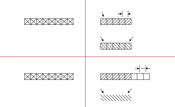
The complex DFT has real and imaginary values both at its input and output. In practice, the imaginary parts of the time domain samples are set to zero. If you are given the output spectrum for a complex DFT, it is useful to know how to relate them to the real DFT output and vice versa. The crosshatched areas in the diagram correspond to points which are common to both the real and complex DFT.

Figure 5.7 shows the relationship between the real and complex DFT in more detail. The real DFT output points are from 0 to N/2, with ImX(0) and ImX(N/2) always zero. The points between N/2 and N – 1 contain the negative frequencies in the complex DFT. Note that ReX(N/2 + 1) has the same value as Re(N/2 – 1). Similarly, ReX(N/2 + 2) has the same value as ReX(N/2 – 2), etc. Also, note that ImX(N/2 + 1) is the negative of ImX(N/2 – 1), and ImX(N/2 + 2) is the negative of ImX(N/2 – 2), etc. In other words, ReX(k) has even symmetry about N/2 and ImX(k) has odd symmetry about N/2. In this way, the negative frequency components for the complex FFT can be generated if you are only given the real DFT components.

The equations for the complex and the real DFT are summarized in Figure 5.8. Note that the equations for the complex DFT work nearly the same whether taking the DFT, X(k) or the IDFT, x(n). The real DFT does not use complex numbers, and the equations for X(k) and x(n) are significantly different. Also, before using the x(n) equation, ReX(0) and ReX(N/2) must be divided by two. These details are explained in Chapter 31 of Reference 1, and the reader should study this chapter before attemping to use these equations.

CONSTRUCTING THE COMPLEX DFT NEGATIVE FREQUENCY COMPONENTS FROM THE REAL DFT

Axis of

Symmetry

Figure 5.7

5.7

FAST FOURIER TRANSFORMS

The DFT output spectrum can be represented in either polar form (magnitude and phase) or rectangular form (real and imaginary) as shown in Figure 5.9. The conversion between the two forms is straightforward.

COMPLEX AND REAL DFT EQUATIONS

Figure 5.8

CONVERTING REAL AND IMAGINARY DFT

OUTPUTS INTO MAGNITUDE AND PHASE

MAG[X(k)]

ϕ

Re X(k)

Figure 5.9

5.8