

Литература / Speech recognition (Steve Renals)
.pdfSPEECH RECOGNITION
Steve Renals
February 1998
COM326/COM646/COM678 |
2 |
COM326/COM646/COM678 |
3 |
Chapter 1
TEMPLATE MATCHING
1.1 Introduction
A well-studied approach to automatic speech recognition is based on the storage of one or more acoustic patterns (templates) for each word in the recognition vocabulary. If the system is speaker-dependent, then these words will have been spoken by the intended user. The recognition process then consists of matching the incoming speech with stored templates.
This process has been most used for isolated word recognition, In that case the input speech consists of an isolated whole word (which has been endpoint detected, typically using an energy-based measure) and this word is matched against each of the stored templates. The template with the lowest distance from the input is the recognised word. In these notes, we'll mainly be considering isolated word recognition.
There are two key issues that need to be dealt with to construct an isolated word recognition system based on template matching:
Features In what form should the speech data be represented? (i.e. what are the feature vectors?)
Distances How do we compute the distances between two speech patterns?
The answer to the second question is crucial. It can be broken down into two parts:
1.How do we compute the local distance between two feature vectors?
2.How do we compute the global distance between two speech patterns (words) from the local distances, given that input word and the template may have different durations/time scales?
1.2Feature Vectors
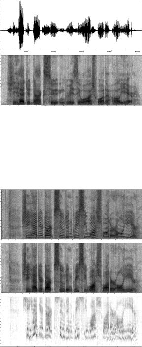
The way data is represented is crucial to speech pattern recognition. As an example consider fig. 1.1. This shows an utterance “She had your dark suit in greasy wash water all year” spoken twice by the same speaker, represented as a time-amplitude waveform and as a spectrogram.
All the information in the spectrogram is in the waveform—further processing will never create new information—b ut the spectrogram seems to contain most of the essential information in a “clearer” way. The feature extraction process might then be regarded as an information reduction process in which “irrele vant” information is thrown away.
Of course there are many possible feature extraction processes e.g. wideband and narrowband FFTs, auditory representations (e.g. based on gammatone filterbank).
COM326/COM646/COM678 |
4 |
Figure 1.1: Waveform and spectrogram representations of “She had your dark suit in greasy wash water all year” spoken by a male speaker
Figure 1.2: Feature extraction processes: narrowband FFT (top), wideband FFT (middle) and auditory filterbank excitation pattern (bottom).
COM326/COM646/COM678 |
5 |
The question of optimal feature extraction is not trivial. If we are interested in recognition, then an ideal feature extractor might be one that produces a string of words (making the rest of the recognizer redundant)! On the other hand, separating the feature extraction process from the pattern recognition process is a sensible thing to do, since it enables us to encapsulate the pattern recognition process.
We shall concern ourselves with frame based feature extraction. That is, the feature analysis consists of computing a feature vector at regular intervals. For example if we perform a filterbank analysis, then our feature vector may consist of the energies in each band averaged over (say) 20ms. For a linear predictive analysis the feature vector consists of the prediction coefficients (or transformations of them). A common feature vector type used in speech recognition are Mel Frequency Cepstral Coefficients (MFCCs), covered in COM325.
1.3 Local Distances
An important operation is the comparison of two input vectors—ho w similar are vectors x and y, or what is the distance between them? In speech recognition we often refer the distance between two frames of data as a local distance, with the overall distance between an input word and a template referred to as a global distance.
We shall use the notation d x y for the local distance between two feature vectors. Two possible choices for a local distance metric are:
The Euclidean distance metric: |
|
|
|
|
|
||
|
|
xi yi 2 |
(1.1) |
||||
d2 x y |
x y T x y |
|
|||||
|
|
|
|
å |
|
|
|
|
|
|
|
i |
|
|
|
where xi is the ith element of x and xT signifies the transpose of x. |
|
||||||
The City Block or Manhattan distance metric: |
|
|
|
|
|
||
d1 x y x y |
xi yi |
(1.2) |
|||||
å |
|
|
|
|
|
||
|
|
i |
|
|
|
|
|
The principal benefit of the City Block metric is that it is computationally cheaper than the Euclidean metric. The Euclidean distance gives more weight to large differences in a single feature (relative to smaller differences in all features) compared with the City Block distance. The Euclidean distance is much more frequently used, particularly as it has certain theoretical properties that arise when it is used in statistically-based speech recognition.
Both these metrics make the implicit assumption that individual elements of a feature vector are not correlated with each other. This is clearly not the case for a simple filter -bank representation – what goes on in one channel is clearly related to what is going on in the neighbouring channel. However cepstral feature vectors do have uncorrelated elements; furthermore, it can be shown that using the Euclidean distance to compare cepstra has several “nice” theoretical properties.
Finally, there are some speech specific distance measures. One of the best known is the Itakura distance which is used with an LPC analysis. This distance is similar in concept to Residual Excited LPC. Essentially the distance measure is the residual that results from using the LPC filter derived from one signal to inverse filter the other.
1.4 Global Distances
Speech is a time-dependent process. Several utterances of the same word are likely to have different durations, and utterances of the same word with the same duration will differ in

COM326/COM646/COM678 |
6 |
the middle, due to different parts of the words being spoken at different rates. To obtain a global distance between two speech patterns (represented as a sequence of vectors) a time alignment must be performed.
This problem is illustrated in figure 1.4, in which a “time-time” matrix is used to visualize the alignment. As with all the time alignment examples the reference pattern (template) goes up the side and the input pattern goes along the bottom. In this illustration the input “SsPEEhH” is a `noisy' version of the template “SPEECH”. The idea is that `h' is a closer match to `H' compared with anything else in the template. The input “SsPEEhH” will be matched against all templates in the system's repository. The best matching template is the one for which there is the lowest distance path aligning the input pattern to the template. A simple global distance score for a path is simply the sum of local distances that go to make up the path.
N
Time
1 j-1 j
H
C
E
E
P
S
|
|
|
|
|
|
|
|
|
|
i-1,j |
i,j |
|
|
|
|
|
|
|
|
|
|
||
|
|
i-1 |
|
i,j-1 |
|
|
|
|
|
|
|
|
|
||
|
|
j-1 |
|
|
|
||
S |
s |
|
|
|
E |
h |
H |
P |
E |
||||||
1 |
|
|
i-1 |
i |
|
|
n |
|
|
|
|
|
|
|
|
|
|
|
|
|
Time |
|
|
Figure 1.3: Illustration of a time alignment path between a template pattern “SPEECH” and a noisy input “SsPEEhH”.
How do we find the best-matching ( lowest global distance) path between an input and a template? We could evaluate all possible paths – but this is extremely inefficient as the number of possible paths is exponential in the length of the input. Instead, we will consider what constraints there are on the matching process (or that we can impose on that process) and use those constraints to come up with an efficient algorithm. The constraints we shall impose are straightforward and not very restrictive:
1.Matching paths cannot go backwards in time;
2.Every frame in the input must be used in a matching path;
3.Local distance scores are combined by adding to give a global distance.
For now we will also extend (2) to say that every frame in the template and the input must be used in a matching path. This means that if we take a point i j in the time-time matrix (where i indexes the input pattern frame, j the template frame), then previous point must have been i 1 j 1 , i 1 j or i j 1 (see figure 1.4). The key idea in dynamic programming is that at point i j we just continue with the lowest distance path from
i 1 j 1 , i 1 j or i j 1 .
COM326/COM646/COM678 |
7 |
This algorithm is known as Dynamic Programming (DP). When applied to templatebased speech recognition, it is often referred to as Dynamic Time Warping (DTW). DP is guaranteed to find the lowest distance path through the matrix, while minimizing the amount of computation. The DP algorithm operates in a time-synchronous manner: each column of the time-time matrix is considered in succession (equivalent to processing the input frame-by-frame) so that, for a template of length N, the maximum number of paths being considered at any time is N.
Exercise: Make sure you can convince yourself of this.
If we denote the global distance score up to i j as D i j and the local distance score at that point as d i j , then we can express dynamic programming using the following relation:
D i j min D i 1 j 1 D i 1 j!D i j 1#"%d$i j |
(1.3) |
Given that D 1 1 d 1 1 (this is the initial condition), we have the basis for an efficient recursive algorithm for computing D i j . The final global distance D n N gives us the overall matching score of the template with the input. The input word is then recognized as the word corresponding to the template with the lowest matching score. (Note that N will be different for each template.)
For basic speech recognition DP has a small memory requirement, the only storage required by the search (as distinct from the templates) is an array that holds a single column of the time-time matrix.
Exercise: Show this is so.
If it is required to trace back along the best-matching path (rather than just knowing the score at the end of it) then a backtrace array (or backpointer array) must be kept with entries in the array pointing to the preceding point in that path.
1.5 Extensions to Basic DP
Although the basic DP algorithm (1.3) has the benefit of symmetry (i.e. all frames in both input and reference must be used) this has the side effect of penalising horizontal and vertical transitions relative to diagonal ones.
EXERCISE: Convince yourself that this is so by considering the different ways of going from i 1 j 1 to i j .
One way to avoid this effect is to double the contribution of d i j when a diagonal step is taken. This has the effect of charging no penalty for moving horizontally or vertically rather than diagonally. This is also not desirable (why?), so independent penalties dh and dv can be applied to horizontal or vertical moves. In this case (1.3) becomes:
D i j min D i 1 j 1&$2d i j D i 1 j&$d i j'$dh D i j 1&$d i j&$dv"
(1.4)
Suitable values for dh and dv may be found experimentally.
This approach will favour shorter templates over longer templates, so a further refinement is to normalize the final distance score by template length to redress the balance.
If we restrict the allowable path transitions to be: |
|
|||
i |
1 |
j 2 |
i j (skips a template frame – |
diagonal slope 2) |
i |
1 |
j 1 |
)(i j (usual diagonal – slope 1) |
|
i 1 |
j(i j (duplicates a template frame – |
slope 0) |
||
then we are assume that each frame of the input pattern is used once and only once. This means that we can dispense with template-length normalization and it is not required to add
COM326/COM646/COM678 |
8 |
the local distance in twice for diagonal (slope 1) path transitions. This approach is referred to as asymmetric dynamic programming (in contrast to the version in figure 1.4 which is symmetric).
Dynamic programming may be regarded as an efficient algorithm to perform an exhaustive search. This means that it will always find the path with the lowest global distance when matching an input with a template, and will be a lot more efficient than exhaustive search. However, there can still be a lot of computation, particularly when there are many templates to compare an input pattern against. A significant saving in computation can be made if pruning is employed – this is sometimes called beam search. The basic idea of pruning is very simple: poorly scoring paths (i.e., those paths whose global distance is further away from the lowest distance path at that time) are pruned from the search. This is illustrated in figure 1.4. Pruning is a heuristic, which means it does not guarantee that the algorithm will find the minimum distance path. An example of this situation is given in figure 1.5 in which the input pattern is very poorly matched to the template and if pruning had been employed, the best scoring path would not have been found.
Figure 1.4: An example of DP search using the asymmetric approach together with path pruning.
COM326/COM646/COM678 |
9 |
Figure 1.5: An example of DP search comparing an input (”three”) with a dissimilar template (”eight”). This is an example of a case where the final lowest distance path would have been pruned mid-utterance. The path marked by crosses was the lowest distance until the final frame.

COM326/COM646/COM678 |
10 |
1.6 Connected Word Recognition
So far we have considered dynamic programming as an algorithm for isolated word recognition. However it is quite possible to generalize the algorithm to the case of connected word recognition. In this case a point in the search space is represented by three indicesi j k , representing frame i of the input, frame j of template k — unlike isolated word recognition where one template is processed at a time, in connected word recognition the word template being processed is a variable to keep track of (figure 1.6). The best path through the word templates k can be found in the same way as for isolated word recognition. However, the start and end points of the templates are not known so for every input frame when a valid path reaches the end of a template k1, a new template k2 might begin.
i
 (i,j,3)
T3
j
T2
T1
word1 |
word2 |
word3 |
|
|
|
Figure 1.6: Dynamic programming for connected word recognition.
The global distance of a path is kept in the usual way; it is the distance summed over all templates the path has passed through, so the distance for individual templates is not recorded. This means that template duration normalization is not possible, so asymmetric dynamic programming should be used.
If paths through two (or more) templates reach the template end at the same frame, then only one of those paths can be extended by starting a new template (figure 1.7).
Exercise: Why is this so?
Which path should be chosen? The answer is provided by the dynamic programming principal: choose the past with the lowest global distance. We can represent this in the