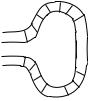
where the collar is indicated in the figure. We obtain a homeomorphism Φ : UN −→ N × G mapping α1(x, s, t) to (x, β1(s, t)) and α2(x, s, t) to (x, β2(s, t)). The map Φ is an isomorphism of stratifolds outside N. By construction the collar induced from N × G via Φ and the collars of W1 along ∂W1 − im ϕY1 and of W2 along ∂W2 − im ϕY2 fit together to give a collar on W1 Z W2 finishing the proof of:

Proposition A.1. For i = 1, 2 let Wi be c-stratifolds such that ∂Wi is obtained by gluing two c-stratifolds Z and Yi over the common boundary

∂Z = ∂Yi = N:

∂Wi = Z N Yi.

Choose representatives of the germs of collars for Yi and Z.

Then there is a c-stratifold W1 Z W2 extending the stratifold structures on Wi − (Z im ϕYi ). The boundary of W1 Z W2 is Y1 N Y2.

It should be noted that the construction of the collar of W1 Z W2 depends on the choice of representatives of the collars of Wi, Yi and Z. For our application in the proof of the Mayer-Vietoris sequence it is important to observe that the collar was constructed in such a way that, away from the neighbourhood of the union of the collars of N in Yi and Z, it is the original collar of W1 and W2.

3. Proof of Proposition 4.1

We conclude this appendix by proving that for a space X the isomorphism classes of pairs (S, g), where S is an m-dimensional stratifold, and g : S → X is a continuous map, form a set.

Proof of Proposition 4.1: For this we first note that the di eomorphism classes of manifolds form a set. This follows since a manifold is di eomorphic to one obtained by taking a countable union of open subsets of Rm (the domains of a countable atlas) and identifying them according to an appropriate equivalence relation. Since the countable sum of copies of Rm forms a set, the set of subsets of a set forms a set, and the possible equivalence relations on these sets form a set, the di eomorphism classes of m-dimensional

manifolds are a subset of the set of all sets obtained from a countable disjoint union of subsets of Rm by some equivalence relation.

Next we note that a stratifold is obtained from a disjoint union of manifolds, the strata, by introducing a topology (a collection of certain subsets) and a certain algebra. The possible topologies as well as the possible algebras are a set. Thus the isomorphism classes of stratifolds are a set. Finally for a fixed stratifold S and space X the maps from S to X are a set, and so we conclude that the isomorphism classes of pairs (S, g), where S is an m-dimensional stratifold, and g : S → X is a continuous map, form a set. q.e.d.

198 B. The detailed proof of the Mayer-Vietoris sequence

(ρ )−1(−∞, − ) ρ−1(−∞, 0) and (ρ )−1( , ∞) ρ−1(0, ∞).

If ∂T = , then (T, id) and (T , f) are bordant.

Proof: Choose δ > 0 such that such that (−δ, δ) consists only of regular values of ρ.

Consider a monotone smooth map μ : R → R which is the identity for |t| > δ/2 and 0 for |t| < δ/4.

μ

Then η : T × R → R mapping (x, t) → ρ(x) − μ(t) has 0 as a regular value. Namely, for those (x, t) mapping to 0 with |t| < δ we have |ρ(x)| < δ and thus (x, t) is a regular point of η, and for those (x, t) mapping to 0 with |t| > δ/2 we have μ(t) = t and again (x, t) is a regular point. Thus

To relate T to T, consider the map f : T → T given by the restriction of the projection onto T in T × R. This is an isomorphism outside ρ−1(0) × (−δ/2, δ/2). In particular we can identify the boundaries via this isomorphism: ∂T = ∂T. Similarly we use this isomorphism to induce a collar on T from a small collar of T and so the c-structure on T makes T a regular c-stratifold. Finally we define ρ by the projection onto R. The desired properties are obvious and this finishes the proof of the first statement.

If ∂T = , we want to construct a bordism between (T, id) and (T , f). For this, choose a smooth map ζ : I → R which is 0 near 0 and 1 near

1. Then consider the smooth map T × R × I → R mapping (x, t, s) → ρ(x) − (ζ(s)μ(t) + (1 − ζ(s))t). This map again has 0 as regular value and the preimage of 0 is the required bordism Q. By construction and Proposition 4.2 Q is a regular c-stratifold. The projection from Q to T is a map r : Q → T, whose restriction to T is the identity on T and whose restriction to T is f. Thus (Q, r) is a bordism between (T, id) and (T , f).

q.e.d.

Now we apply this lemma to the proof of Proposition 5.1 and the detailed proof of Theorem 5.2, the Mayer-Vietoris sequence.

Proofs of Proposition 5.1 and Theorem 5.2: We begin with the proof of Proposition 5.1. For [S, g] SHm(X) we consider (as before Proposition 5.1) the closed subsets A := g−1(X − V ) and B := g−1(X − U). Using a

partition of unity we construct a smooth function ρ : S → R and choose a regular value s such that ρ−1(s) S − (A B) and A ρ−1(s, ∞) and B ρ−1(−∞, s). After composition with an appropriate translation we can assume s = 0. Since S is compact, by Proposition 4.3 the regular values of ρ form an open set in R.

Thus we can apply Lemma B.1 and we consider S , f and ρ . Then (S, g) is bordant to (S , gf) (since (S , f) is bordant to (S, id)) and 0 is a regular value of ρ . By construction, ρ−1(0) × (− , ) is contained in S as open neighbourhood of P := (ρ )−1(0) = ρ−1(0), in other words we have a bicollar of P. Furthermore by construction gf is equal to g on P = ρ−1(0), in particular, gf(P) is contained in U ∩ V . In Proposition 5.1 we defined

d([S, g]) as [ρ−1(0), g|ρ−1(0)] and the considerations so far imply that this definition is the same if we pass from (S, g) to the bordant pair (S , gf) and

define d([S , gf]) as [P, gf|P]: this situation has the advantage that P has a bicollar.

To show that d is well defined it is enough to show that if (S , gf) is the boundary of (T, F ), then [P, g|P] is zero in SHk−1(U ∩ V ). Here T is a c-stratifold with boundary S . In particular we can take as T the cylinder over S and see that d does not depend on the choice of the separating function or the regular value. We choose a representative of the germ of collars c of T. Define AT := F −1(A) and BT := F −1(B) and construct a smooth function η : T → R with the following properties:

1)There is a μ > 0 such that the restriction of η to P × (−μ, μ) is the projection to (−μ, μ),

2)η(c(x, t)) = η(x),

200 B. The detailed proof of the Mayer-Vietoris sequence

3) there is an δ > 0 such that F (η−1(−δ, δ)) U ∩ V .

The construction of such a map η is easy using a partition of unity since P has a bicollar in S .

By Sard’s theorem there is a t with |t| < min{δ, μ} which is a regular

guarantee that Q := η−1(t) is a c-stratifold with boundary P × {t}. By con-

dition 3) we know that F (Q) U ∩ V and so we see that [P × {t}, F |P×{t}] is zero in SHk−1(U ∩ V ). On the other hand, obviously [P × {t}, F |P×{t}] is bordant to [P, g|P]. This finishes the proof of Proposition 5.1.

Now we proceed to the proof of Theorem 5.2. We first show that d commutes with induced maps. The reason is the following. Let X be a space with decomposition X = U V and h : X → X a continuous map respecting the decomposition. Then if we consider (S, hf) instead of (S, f),

one can take the same separating function ρ in the definition of d and so d ([S, hf]) = [ρ−1(s), hf|ρ−1(s)] = h ([ρ−1(s), f|ρ−1(s)]) = h (d([S, f])).

Now we begin the proof of the exactness by examining

SHn(U ∩ V ; Z/2) → SHn(U; Z/2) SHn(V ; Z/2) → SHn(U V ; Z/2).

Since jU iU = i : U ∩ V → U V , the inclusion map, and also jV iV = i, the di erence of the composition of the two maps is zero. To show the re-

verse inclusion, consider [S, f] SHn(U; Z/2) and [S , f ] SHn(V ; Z/2) with (jU ) ([S, f]) = (jV ) ([S , f ]). Let (T, g) be a bordism between [S, f] and [S , f ], where g : T → U V . Similarly, as in the proof that d is well defined, we consider the closed disjoint subsets AT := S g−1(X − V ) and BT := S g−1(X − U). Using a partition of unity we construct a

smooth function ρ : T → R with ρ(A) = −1 and ρ(B) = 1 and choose a

◦

regular value s such that ρ−1(s) T − (AT BT). After composition with an appropriate translation we can assume s = 0. Since T is compact, by Proposition 4.3, the regular values of ρ form an open set in R. Applying Lemma B.1 we can assume after replacing T by T that ρ−1(s) has a bicol-

lar ϕ. Then [ρ−1(s), g|ρ−1(s)] SHn(U ∩ V ) and — as explained in §3 — (ρ−1[s, ∞), g|ρ−1[s,∞)) is a bordism between (S, f) and (ρ−1(s), g|ρ−1(s)) in U.

Similarly we obtain by (ρ−1(−∞, s]), g|ρ−1(−∞,s])) a bordism between (S , f ) and (ρ−1(s), g|ρ−1(s)) in V . Thus

((iU ) ([ρ−1(s), g|ρ−1(s)]), (iV ) ([ρ−1(s), g|ρ−1(s)])) = ([S, f], [S , f ]).

Next we consider the exactness of

d

SHn(U V ; Z/2) → SHn−1(U∩V ; Z/2) → SHn−1(U; Z/2) SHn−1(V ; Z/2).

By construction of the boundary operator the composition of the two maps is zero. Namely (ρ−1[s, ∞), f|ρ−1[s,∞)) is a null cobordism of d([S, f]) in U and (ρ−1(−∞, s], f|ρ−1(−∞,s]) is a zero-bordism of d([S, f]) in V . Here we again apply Lemma B.1 and assume that ρ−1(s) has a bicollar.

To show the reverse inclusion, start with [P, r] SHn−1(U ∩V ; Z/2) and suppose (iU ) ([P, r]) = 0 and (iV ) ([P, r]) = 0. Let (T1, g1) be a zero bordism of (iU ) ([P, r]) and (T2, g2) be a zero bordism of (iV ) ([P, r]). Then we consider T1 PT2. Since g1|P = g2|P = r, we can, as in the proof of the transitivity of the bordism relation, extend r to T1 P T2 using g1 and g2 and denote this map by g1 g2. Thus [T1 P T2, g1 g2] SHn(U V ; Z/2). By the construction of the boundary operator we have d([T1 PT2, g1 g2]) = [P, r]. Using the bicollar one constructs a separating function which near P is the projection from P × (− , ) to the second factor.

Finally, we prove exactness of

d

SHn(U; Z/2) SHn(V ; Z/2) → SHn(U V ; Z/2) → SHn−1(U ∩ V ; Z/2).

The composition of the two maps is obviously zero. Now, consider [S, f] SHn(U V ; Z/2) with d([S, f]) = 0. Consider ρ, s and P as in the definition of the boundary map d and assume by Lemma B.1 that ρ−1(s) has a bicollar. We put S+ := ρ−1[s, ∞) and S− := ρ−1(−∞, s]. Then S = S+ P S−. If d([S, f]) = [P, f|P] = 0 in SHn−1(U ∩ V ; Z/2) there is Z with ∂Z = P and an extension of f|P to r : Z → U ∩ V . We glue to obtain S+ P Z and S− P Z. Since f|P = r|P the maps f|S+ and r give a continuous map f+ : S+ P Z → U and similarly we obtain f− : S− P Z → V . We are

finished if (jU ) ([S+ P Z, f+]) − (jV ) ([S− P Z, f−]) = [S, f]. For this we have to find a bordism (T, g) such that ∂T = S+ Z + S− Z + S (recall that −[P, r] = [P, r] for all elements in SHn(Y ; Z/2)) and g extends the given three maps on the pieces.

This bordism is given as T := ((S+ P Z) × [0, 1]) Z ((S− P Z) × [1, 2])

with ∂T = (S+ P Z) × {0} + (S− P Z) × {2} + S+ P S−. Here we apply Lemma A.1 to smooth the corners or cusps. This finishes the proof of The-

orem 5.2. q.e.d.

Finally we discuss the modification needed to prove the Mayer-Vietoris sequence in cohomology. Everything works with appropriate obvious modifications as for homology except where we argue that the regular values of the separating map ρ form an open set. This used the fact that the stratifold on which ρ is defined is compact, which is not the case for regular stratifolds representing cohomology classes. The separating function can be chosen as we wish, and we show now that we can always find a separating function ρ and a regular value, which is an interior point of the set of regular values.

Let g : S → M be a proper smooth map and C and D be disjoint closed subsets of M. We choose a smooth map ρ : M → R which on C is 1 and on D is −1. We select a regular value s of ρg. The set of singular points of ρg is closed by Proposition 4.3, and since a proper map on a locally compact space is closed [Sch, p. 72], the image of the singular points of ρg under g is a closed subset F of M.

Now we consider a bicollar ϕ : U → M −F of ρ−1(s), where U = {(x, t) ρ−1(s) × R | |t| < δ(x)} for some continuous map δ : ρ−1(s) → R>0. We can choose ϕ in such a way that ρϕ(x, t) = t. Now we “expand” this bicollar by choosing a di eomorphism from U to ρ−1(s) × (−1/2, 1/2) mapping (x, t) to (x, η(x, t)), where η(x, ·) is a di eomorphism for each x ρ−1(s). Using this, it is easy to find a new separating function ρ , such that ρ ϕ(x, t) = t and ρ −1(−1/2, 1/2) = U. By construction the interval (−1/2, 1/2) consists only of regular values of ρ f.

We apply this in the proof of the Mayer-Vietoris sequence for cohomology as follows. Let U and V be open subsets of M = U V . We consider the closed subsets C := M − U and D := M − V . Then we construct ρ as above and note that ρ g is a separating function of A := g−1(C) and B := g−1(D), and s is a regular value which is an interior point of the set of

regular values. With this the definition of the coboundary operator works as explained in chapter 12.

Now we explain why the Mayer-Vietoris sequence is exact. We shall explain each argument in figuress, with a brief description followed by a sequence of four figures presented on the immediately following page.

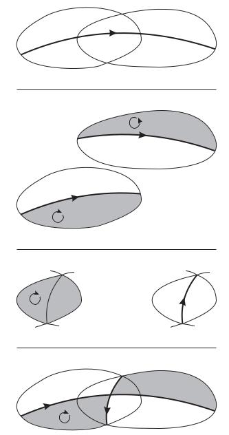
We begin with the exactness of

SHk−1(U ∩ V ) → SHk(U V ) → SHk(U) SHk(V ).

Let α SHk(U V ) (figure A) such that it maps to zero, i.e., there are stratifolds with boundary and proper maps extending the map representing α after restricting to U and V respectively. We abbreviate these extensions by β and γ and write ∂β = jU (α) and ∂γ = jV (α) (figure B). Now we restrict β and γ to the intersection U ∩ V and glue them (respecting the orientations) along the common boundary to obtain ζ := (−γ|U∩V ) β|U∩V SHk−1(U ∩V ) (figure C). Using a separating function ρ we determine the image of ζ under the coboundary operator: δ(ζ). Finally we have to show that

δ(ζ) is bordant to α. For this we consider η := β|ρ−1(−∞,s] (−γ|ρ−1[s, ∞)), which gives such a bordism (figure D).

A

V

U

α SHk(U V )

B

γ

jV α = ∂γ

jU α = ∂β

β

D

η := β| −1(−∞,s]

(−γ| −1[s,∞))

∂η = α − δζ

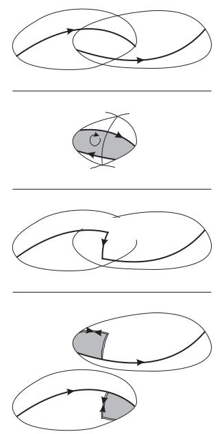
Now we consider the exactness of the sequence (see next page for figures)

SHk(U V ) → SHk(U) SHk(V ) → SHk(U ∩ V ).

For this we consider α SHk(U) and β SHk(V ) (figure A) such that (α, β) maps to zero in SHk(U ∩ V ). This means there is γ, a stratifold with boundary together with a proper map to U ∩V , such that ∂γ = iU (α)−iV (β) (figure B). Next we choose a separating function ρ as indicated in figure B.

Using ρ we consider ζ := α| −1(−∞,s] (−δγ) β| −1[s,∞) SHk(U V ) (figure C). Finally we have to construct a bordism between jU (ζ), and α

Finally we consider the exactness of the sequence (see next page for figures)

SHk(U) SHk(V ) → SHk(U ∩ V ) → SHk+1(U V ).

Let α be in SHk(U ∩ V ) (and ρ a separating function) such that δα = 0 (figure A). This means that there is a stratifold β with boundary δ(α) and a proper map extending the given map (figure B). From this we construct the classes ζ1 := α| −1(−∞,s] β|U SHk(U) and ζ2 := (−α| −1[s,∞)) (−β|V ) SHk(V ) (figure C). Finally we note that iU (ζ1) − iV (ζ2) = α (figure D).

A

α SHk(U ∩ V )

−1(s)

U ∩ V

B

β

C

ζ2 :=

(−α| −1 [s,∞)) (−β|V )

ζ1 := α| −1(−∞,s] β|U

D

iU (ζ1) − iV (ζ2) = α

Let K be the submodule generated by these elements. Then we define the tensor product

Remark: The following rules are translations of the relations and very useful for working with tensor products:

r· (v w) = (r · v) w = v (r · w) v w + v w = (v + v ) w

v w + v w = v (w + w ).

These rules imply that the following canonical map is well defined and bilinear:

Let f : V × W → P be bilinear. Then f induces a linear map

This map is well defined since (rv) w−v (rw) → f(rv, w)−f(v, rw) = r f(v, w) − r f(v, w) = 0 and v w + v w − (v + v ) w → f(v, w) + f(v , w) − f(v + v, w) = 0 , respectively, v w + v w − v (w + w ) → 0.

In turn, if we have a linear map from V R W to P , the composition of the canonical map with this map is a bilinear map from V × W to P . Thus as indicated above we have seen the fundamental fact:

The linear maps from V R W to P correspond isomorphically to the bilinear maps from V × W to P .

What is (V V ) R W ? The reader should convince himself that the following maps are bilinear:

and these are inverse to each other. Thus we have shown:

Thus dim Rn R Rm = n · m and

Rn Rm Rn·m M(n, m)

R = =

ei ej −→ ei,j

where ei,j denotes the n × m matrix whose coe cients are 0 except at the place (i, j) where it is 1.

Example:

If R = Z, a Z-module is the same as an abelian group. For abelian groups A and B we write A B instead of A Z B.

We want to determine Z/n Z/m. We prepare this by some general considerations. Let f : A → B and g : C → D be homomorphisms of R-modules. They induce a homomorphism

f g : A R C → B R D

a c → f(a) g(c),

called the tensor product of f and g.

If we have an exact sequence of R-modules

· · · → Ak+1 → Ak → Ak−1 → · · ·

and a fixed R-module P , we can tensor all Ak with P and tensor all maps in the exact sequence with id on P , and obtain a new sequence of maps

· · · → Ak+1 R P → Ak R P → Ak−1 R P → · · ·

called the induced sequence and ask if this is again exact. This is, in general, not the case and this is one of the starting points of homological algebra, which systematically investigates the failure of exactness. Here we only study a very special case.

Proposition C.2. Let

0 → A → B → C → 0

be a short exact sequence of R-modules. Then the induced sequence

A R P → B R P → C R P → 0

is again exact. In general the map A R P → B R P is not injective.

Proof: Denote the map from A → B by f and the map from B to C by g. Obviously (g id)(f id) is zero. Thus g id induces a homo-

morphism B R P/(f id)(A RP ) → C R P . We have to show that this is an isomorphism. We give an inverse by defining a bilinear map C × P to

B R P/(f id)(A RP ) by assigning to (c, p) an element [b p], where g(b) = c. The exactness of the original sequence shows that this induces a well defined

homomorphism from C R P to B R P/(f id)(A RP ) and that it is an inverse of B R P/(f id)(A RP ) → C R P .

The last statement follows from the next example. q.e.d.

As an application we compute Z/n Z/m. For this consider the exact sequence

0 → Z → Z → Z/n → 0

where the first map is multiplication by n, and tensor it with Z/m to obtain an exact sequence

Z Z/m → Z Z/m → Z/n Z/m → 0

Proof: The case of a free finitely generated abelian group P can be reduced to the case P = Z by Proposition C.1. The conclusion now follows

from the isomorphism A Z A.

=

If P = Q we return to Proposition C.2 and note that we are finished if we can show the injectivity of f id : A Q → B Q. Consider an element

q.e.d.