

Кононов / 9
.pdfSingle molecule spectroscopy
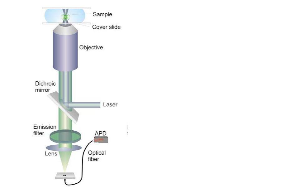
Schematic representation of a (simple) confocal microscope setup. From http://www.microscopyu.com
Confocal scanning microscopy. A parallel laser beam is deflected by a dichroic mirror and focused by a high-numerical aperture objective onto a diffraction-limited spot. The fluorescence signal then passes through the dichroic mirror, is focused onto a pinhole and finally reaches the (point) detector (i.e. a photomultiplier or an avalanche photodiode [APD]). The excitation volume is confined in the x–y plane by focusing; the z-resolution in the detection pathway is provided by the aperture, which blocks light emanating from regions not in the immediate vicinity of the focal volume. Sequential scanning in two or even three dimensions is controlled by a
computer, which also calculates the final image.

Fluorescence Correlation Spectroscopy
Fluorescence correlation spectroscopy (FCS) has recently experienced growing popularity in biochemical and biophysical applications due to significantly improved signal-to-background ratios. The parameters determinable by FCS in intracelluar environment include:
•Fluorescent species (e.g., GFP, beads, dye molecules) diffusion coefficients
•Fluorescent molecules concentration
•Kinetic information of binding and aggregation processes
•Kinetic information of conformation transitions
|
|
Sample |
|
|
Autocorrelation Function |
|
||||||||||||||
|
|
|
Objective |
|
|
|
|
|
|
|
|
|
|
|
|
|
|
|||
|
|
|
|
|
|
|
|
|
|
|
|
|
|
|
|
|
||||
|
|
|
|
|
|
|
|
|
|
|
|
|
|
|
|
|
|
|
Computer |
|
|
|
|
|
|
|
|
|
|
|
|
|
|
|
|
|
|
|
|
||
|
|
|
|
|
|
|
|
|
|
|
|
|
|
|
|
|
|
|
||
|
|
|
|
|
|
|
|
|
|
|
|
|
|
|
|
|
|
|
||
|
|
Dichroic Mirror |
|
|
|
|
|
|
||||||||||||
|
Ti:Sapphire |
|
|
|
|
|||||||||||||||
|
|
|
|
|
|
|
|
|||||||||||||
|
|
|
|
|
|
|
APD |
|
|
|
|
|||||||||
|
Laser |
|
|
|
|
|
||||||||||||||
|
|
|
|
|
|
|
|
|
|
|
|
|
|
|
|
|
|
|
Correlator |
|
|
|
|
|
|
|
|
|
|
|
|
|
|
|
|
|
|
|
|
||
|
|
|
|
|
|
|
|
|
|
|
|
|
|
|
||||||
|
Dichroic Mirror |
|
|
|
|
|
|
|
|
|
||||||||||
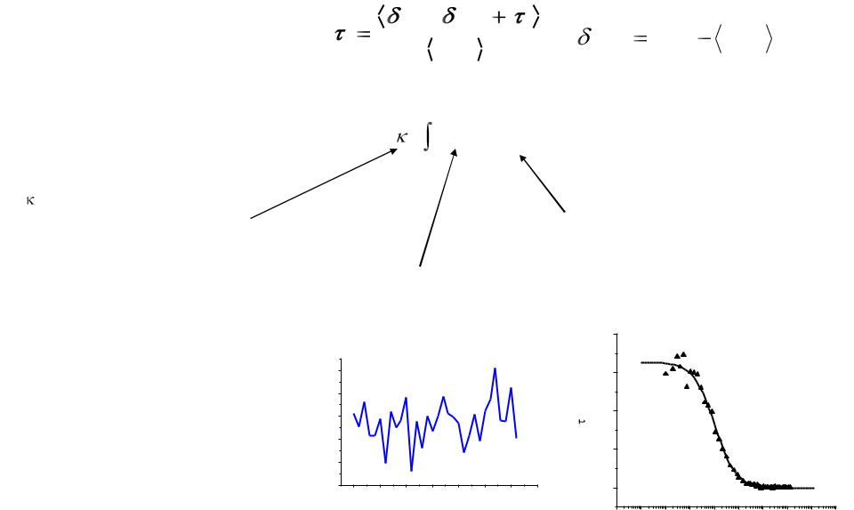
Autocorrelation Function
G( ) |
F(t) F(t |
) |
|
|
|
|
|
|
|
F(t) F(t) F(t) |
|
F(t) |
2 |
|
|||
|
|
|
|
|
|
|
|
|
|
|
|
Factors influencing the fluorescence signal:
Q = quantum yield and detector sensitivity (how bright is our probe). This term could contain the fluctuation of the fluorescence intensity due to internal processes
F(t)  Q dr W (r)C(r,t)
W(r) describes our observation volume
C(r,t) is a function of the fluorophore concentration over time. This is the term that contains the
“physics” of the diffusion processes
(kcps) |
19.8 |
|
|
|
|
|
|
|
|
|
|
|
|
|
|
|
|
||
Intensity |
19.6 |
|
|
|
|
|
|
|
|
19.4 |
|
|
|
|
|
|
|
||
19.2 |
|
|
|
|
|
|
|
||
Detected |
|
|
|
|
|
|
|
||
19.0 |
|
|
|
|
|
|
|
||
18.8 |
|
|
|
|
|
|
|
||
0 |
5 |
10 |
15 |
20 |
25 |
30 |
35 |
||
|
Time (s)
0.4 |
|
|
|
|
0.3 |
|
|
|
|
0.2 |
|
|
|
|
G( ) |
|
|
|
|
0.1 |
|
|
|
|
0.0 |
|
|
|
|
10-9 |
10-7 |
10-5 |
10-3 |
10-1 |
|
|
Time(s) |
|
|

Various parameters can be extracted from the autocorrelation curves. The most prominent are the diffusion coefficient (a–d) (and hence the
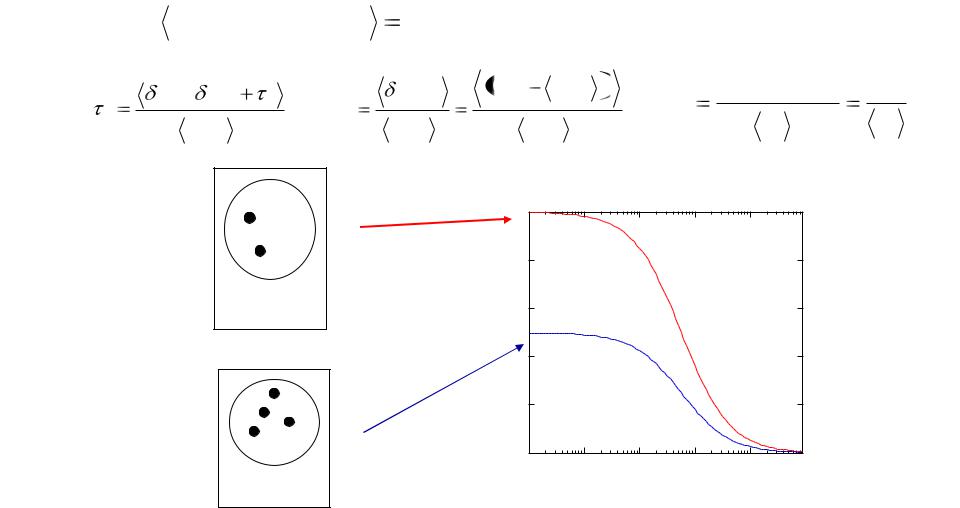
approximate size) and the concentration (e–h) of fluorescent molecules. The half-value decay time provides a good estimate of the mean diffusion time (d), from which the diffusion coefficient can be determined. With increasing mass, the residence time of the molecules in the focal volume is increasing (a–c) and thus the corresponding autocorrelation curves shift to longer diffusion times (d). The amplitude, G(0), is proportional to the inverse particle number and thus to the concentration of the fluorescent particles (e–h). An increase in particle number leads to an increase in average fluorescence (e–g), but the signal change caused by one specific molecule entering or leaving the observation volume becomes less pronounced. This is illustrated in (e,f) by the maximal deviation (arrows) of the idealized fluorescence signal from the mean value (straight line).The autocorrelation amplitude, however, is a measure of fluctuation strength and thus decreases for higher concentrations (h).
Why Is G(0) Proportional to 1/Particle Number?
A Poisson distribution describes the statistics of particle occupancy fluctuations. In a Poissonian system the variance is proportional to the average number of fluctuating species:
|
Particle_Number |
Dispersion |
|
|
|
|
|
|
|||
G( ) |
F (t) F (t |
) |
G(0) |
F (t)2 |
F (t) |
F (t) |
2 |
G(0) |
Dispersion |
1 |
|
F (t) 2 |
|
F (t) 2 |
F (t) 2 |
|
N 2 |
N |
|||||
|
|
|
|
||||||||
|
|
|
|
|
0.5 |
|
|
|
|
|
|
|
|
|
|
|
0.4 |
|
|
|
|
|
|
|
<N> = 2 |
|
0.3 |
|
|
|
|
|
|
||
|
|
|
|
|
|
|
|
|
|
|
|
|
|
|
|
|
G(t) |
|
|
|
|
|
|
|
|
|
|
|
0.2 |
|
|
|
|
|
|
|
|
|
|
|
0.1 |
|
|
|
|
|
|
|
|
|
|
|
0.0 |
|
|
|
|
|
|
|
<N> = 4 |
|
10 -7 |
10 -6 |
|
10 -5 |
10 -4 |
10 -3 |
|
||
|
|
|
|
|
Time (s) |
|
|
||||
|
|
|
|
|
|
|
|
|
|
||

P
P(N F ,T )
FT N e FT
N!
Standart deviation ( ) 
 FT
FT
•Average value <N>= FT
•Approaches a Gaussian distribution as N becomes large
FT=1
1
 N
N  n Ni
n Ni
FT=4
FT=10
N

Antibody - Hapten Interactions
Binding site |
Binding site |
|
carb2
Mouse IgG: The two heavy chains are shown in yellow and light blue. The two light chains are shown in green and dark blue..J.Harris, S.B.Larson, K.W.Hasel, A.McPherson, "Refined structure of an intact IgG2a monoclonal
antibody", Biochemistry 36: 1581, (1997).
Digoxin: a cardiac glycoside used to treat congestive heart failure. Digoxin competes with potassium for a binding site on an enzyme, referred to as potassium-ATPase. Digoxin inhibits the Na-K ATPase pump in the myocardial cell membrane.

Autocorrelation
curves:
Anti-Digoxin Antibody (IgG) Binding to Digoxin-Fluorescein
Digoxin-Fl•IgG
(99% bound)
Digoxin-Fl•IgG
(50% Bound)
Digoxin-Fl
Binding titration from the |
Bound |
|
|
autocorrelation analyses:Ligand |
|
|
Fraction |
120 |
|
|
|
|
100 |
|
|
|
|
80 |
|
|
|
|
60 |
|
|
|
|
40 |
|
|
Kd=12 nM |
|
|
|
|
|
|
20 |
|
|
|
|
0 |
|
|
|
|
10 -10 |
10 -9 |
10 -8 |
10 -7 |
10 -6 |
S. Tetin, K. Swift, & , E, Matayoshi , 2003
[Antibody] free (M)

Raman and IR spectroscopy I. IR spectroscopy