

Image_slides / part4_pca
.pdfLagrangian
|
@L |
|
|
|
m |
|
m |
|
|
|
Xi |
|
X |
||
|
|
|
|
|
|||
|
@w |
|
= w |
i yi xi = 0 ! w = i yi xi (1) |
|||
|
|
|
|
|
=0 |
|
i=0 |
|
|
|
@L |
m |
|
m |
|
|
|
|
Xi |
|
X |
||
|
|
|
|
= |
! |
||
|
|
|
@b |
i yi = 0 |
i yi = 0 (2) |
||
|
|
|
|
|
=0 |
|
i=0 |
Iw is linear combination of training set vectors those i 6= 0 (support vectors)
IUsing (1) and (2) we can get
^ |
m |
1 |
m m |
|
||
L( ) = |
Xi |
|
|
|
XX |
max |
|
i 2 |
i j yi yj hxi ; xj i ! |
||||
|
=1 |
|
||||
|
|
|
|
i=1 j=1 |
|
|
i 0; i = 1; ; m
m
X
i yi = 0
i=0
Support Vector Machine

Obtaining Parameters
ISolving with respect to each i and using (1) obtain w
ITo nd b we can calculate average w xi over all support vectors
INote that
m |
!T |
m |
XX
wT x + b = |
i yi xi x + b = i yi hxi ; xi + b |
i=0 |
i=0 |
Support Vector Machine

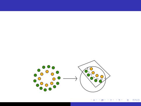
Kernels
IThe algorithm can be written in terms of the inner products hx; zi
IWe could replace all those inner products with h (x); (z)i
IWhere (x) some feature mapping e.g.
0 1 x
(x) = @x2A x3
ISpeci cally, given a feature mapping , we de ne corresponding Kernel to be
K (x; z) = (x)T (z)
Support Vector Machine

Kernel Example
K (x; z) = (xT z)2
|
|
xi zi ! |
0 |
|
1 |
|
|
|
K (x; z) = |
n |
n |
xj zj |
A |
= |
n n |
(xi xj )(zi zj ) |
|
|
Xi |
|
@X |
|
|
XX |
|
|
|
=1 |
|
j=1 |
|
|
|
i=1 j=1 |
|
So this shows that we could split kernel in the product of two maps. The feature map in this case is
|
0x1x1 |
1 |
(x) = |
x1x2 |
|
Bx1x3C |
||
|
B |
C |
|
B |
C |
|
Bx3x3C |
|
|
@ |
A |
where n = 3
Support Vector Machine
Polynomial Kernel
K (x; z) = (xT z + c)d
I This kernel corresponds to a feature mapping to an n+d
d
dimensional space
IComputing K (x; z) takes time O(n) while computing of feature maps takes at least O(nd )
Support Vector Machine

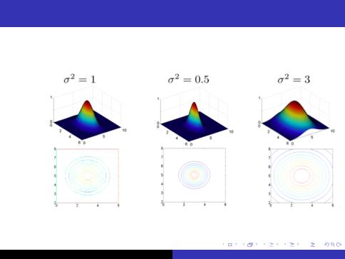
Gaussian Kernel
ILet's think about kernels as measure of similarity between two feature maps
Iif (x) and (z) are close together then product of(x)T (x) is large.
Iif (x) and (z) are far apart then product of (x)T (x) is small.
K (x; z) = exp |
jjx zjj2 |
|
|
2 2 |
|||
|
Support Vector Machine
Gaussian Kernel
Support Vector Machine

Kernel Validation
I Let K be also a matrix where each element
Ki;j = K (x(i); x(j))
.
I If K is a valid kernel then
Ki;j = K (x(i); x(j)) = (x(i))T (x(j)) = = (x(j))T (x(i)) = K (x(j); x(i)) = Kj;i
I Moreover for any z we have
XX XX
zT Kz = zi Ki;j zj = zi (x(i))T (x(j))zj =
i j i j
!2
= Xi |
Xj |
Xk |
zi k (x(i))T k (x(j))zj = Xk |
Xi |
zi k (x(i)) |
|||||||||
|
|
|
|
|
|
|
|
|
|
|
|
|
|
|
|
|
|
|
|
|
|
|
|
|
|
|
|||
|
|
|
|
Support Vector Machine |
|
|
|
|
|
|
|
|||
|
|
|
|
|
|
|
|
|
|
|
|
|
|
|

Mercer Theorem
K is a valid kernel () for any fx(1); x(2); :::; x(m)g corresponding kernel matrix K is symmetric positive semi-de nite.
Support Vector Machine
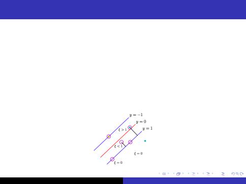
Optimization Task, Soft Margin
IIn case of linearly inseparable case examples are permitted to have margin less then 1
yi (w xi b) 1 i
IIf example has margin 1 i with > 0 we would pay a cost of objective function to being increased by C i
X jjwjj = w wT + C i
i
Support Vector Machine