

Diurnal temperature variation in the boundary layer
The diurnal temperature variation is defined by the variation of the heat influx to the earth’s surface during 24 hour period.
During daytime the earth’s surface is getting heat due to solar radiation influx, and its temperature grows up. During night hours it looses energy due to effective radiation and its temperature grows down.
Recall, that the atmosphere does not directly absorb the solar
radiation. The air’s own radiation at night hasn’t significant impact on the air temperature.
Therefore, the main reason for temperature variation is the eddy exchange with the underlying surface. This process is responsible for the diurnal temperature variation within whole
boundary layer up to 1 - 1,5 km altitude.
1
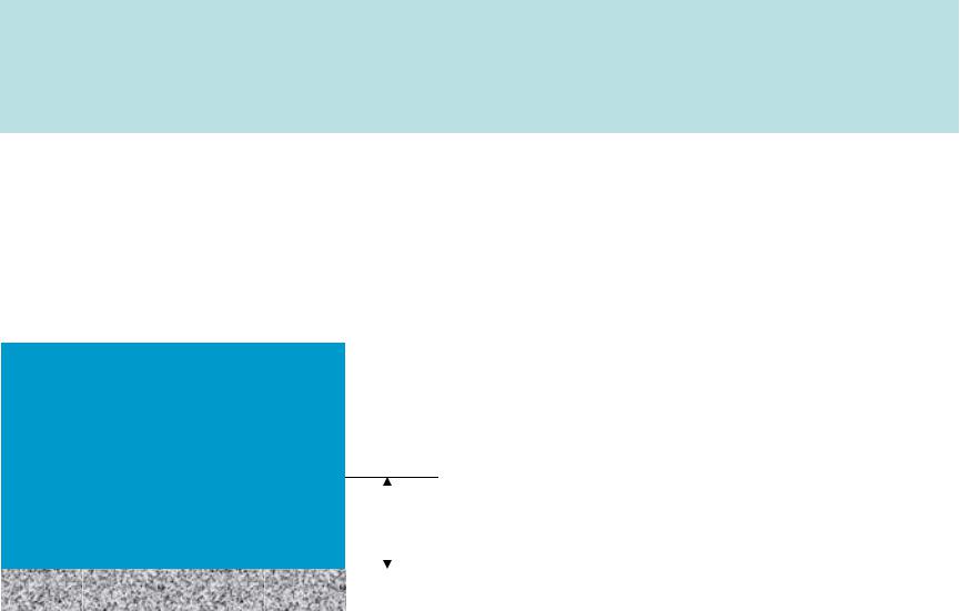
Definition of the boundary layer
Directly adjacent to the underlying surface layer of the atmosphere within which diurnal variation of various atmospheric parameters (temperature, humidity, wind speed, etc) is well defined is called boundary layer of the atmosphere
Free atmosphere
Boundary layer |
|
|
|
|
300-1500m |
||||
|
||||
Surface layer 10 – 250 m |
|
|
|
|
|
|
|
||
|
|
|
||
In tropics, where the atmosphere can be…
extremely unstable, the top of the boundary layer can reach 3000 m.
The height of the boundary layer depends upon static stability of the atmosphere.
Very stable atmosphere
hB.L. 300m
Very unstable atmosphere
hB.L. 1500m
2
Mechanism of the heat spreading up
According to observation, minimal temperatures are observed near the sunrise or a bit later.
Top of the boundary layer
As soon as the solar radiation comes to the surface, the latter starts warming.
Due to molecular diffusion, the heat is transferred to the thin layer of air.
Later the heat is transferred upward due to eddy mixing from one layer to that above of it and so on.
Since for the heat transfer up some period of time is needed, there is delay
with temperature grow in every following layer |
3 |
|

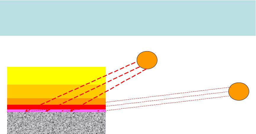
The heat amount, as it spreads up, becomes smaller and smaller because each layer takes some fraction of heat from the ascending heat flux. That makes temperature variation at each following layer smaller and smaller too.
Suppose, there are n layers, the lowest of them (adjacent to the surface) is the well known “surface layer”, where the heat flux is quasi- constant, or well call it zero layer (Q0).
Qn 0 Tn 0
Q3 Q2 |
T |
Q2 Q1 |
3 T |
|
2 |
Q1 Q0 |
T |
Q0 |
1 |
T |
|
|
0 |
The following layers are 1, 2, … n. In every of these layers the heat influx is smaller than in the lower one.
It means that ∆T values will decrease with height.
T0 T1 T2 ... T4n
An example of the diurnal temperature variation
A 150 |
С |
A 12,20 |
С |
0.5 |
|
2 |
|
If we go up, the amplitude will become smaller, and, at the boundary
layer top, it will be close to zero.
5
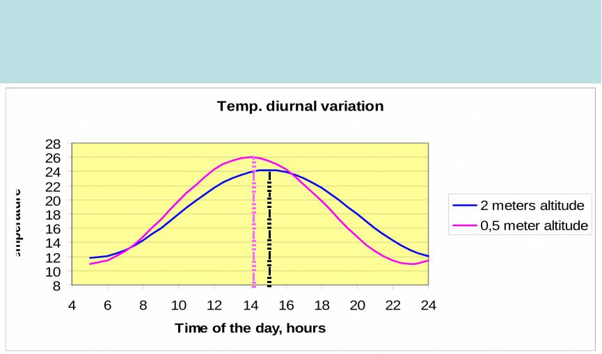
Diurnal temperature variation at different altitudes
1.The amplitude of the variation decreases with height. At the altitude of about 1.5 km it is 6 – 7 times less than near the surface.
2.Near the top of the boundary layer the amplitude can be very
complicated with 2 or 3 maxima.
T |
|
Reasons |
|
2 m |
1. |
Observations are not accurate enough. |
|
2. |
Fluctuation of eddy intensity. |
||
1500tm |
Near the surface, variation is rather significant. Therefore, comparably small fluctuation of eddy intensity do not seriously distort the diurnal temperature variation rate. At the top of the boundary layer, situation is different. Here, the amplitude is much smaller than at the surface, and even not significant eddy activity fluctuation may result in distortion of
the diurnal variation rate.
6
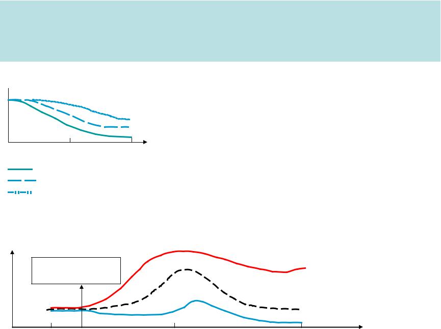
Cloudiness and wind impact on the diurnal temperature variation
 A
A
Cloudiness
|
|
An increase of the cloud amount always |
|
0.5 |
1 |
results in decrease of the diurnal |
|
temperature variation amplitude |
|||
Cloud amount |
|
||
|
|
Low clouds
Middle clouds Wind Upper clouds
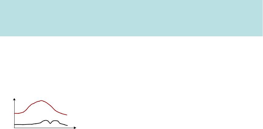
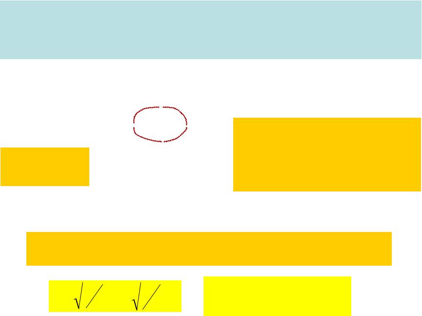
Wind makes the eddy mixing more intensive, and by this way it diminishes the variation amplitude. Along with this, it is associated with temperature advection that also distorts the rate of the variation.
T Starting moment |
|
Warm advection |
|
|
of advection |
|
|
||
|
|
|
|
|
|
|
No advection |
|
|
|
|
Cold advection |
|
|
S.R |
Noon |
S.S |
t |
7 |
|
||||
Simplified theory of the diurnal temperature variation
|
T |
|
K |
T ' z,t ; |
K const; |
|
|
K T ' z,t |
|||||||||||||
|
|
z |
|||||||||||||||||||
|
|
|
|||||||||||||||||||
|
t |
z |
|
z |
|
|
|
|
|
z |
|||||||||||
|
|
|
|
|
z |
|
z,t |
|
|
|
|
|
|||||||||
|
T z,t T |
|
|
|
|
|
|
|
|
||||||||||||
|
|
|
|
|
Boundary conditions |
||||||||||||||||
|
|
|
|
||||||||||||||||||
|
|
|
|
|
|
|
|
|
|
|
|
|
z 0 |
||||||||
|
|
|
|
|
|
Partial differential |
|||||||||||||||
|
|
equation of the |
|
|
|
|
|||||||||||||||
t |
z K |
z |
|
z z0 |
t A0COS t |
||||||||||||||||
|
second order |
|
|||||||||||||||||||
At the given boundary conditions, the solution of the equation will be:
A0 exp az COS t az
|
|
|
|
|
|
|
2 |
|
a |
|
2K |
|
|
K |
7.29 10 5 s 1 |
||
|
|
|
|
|
8 |
|||
|
|
|
|
|
|
|
||
|
|
|
|
|
|
|
|
|
A z


 COS t az
A z A0 exp az Amplitude variation with height
Suppose, we took two altitudes
same value. |
|
|
|
|
|
|
|
|
|
|
|
|
|||
A z1 |
|
z1 |
|
|
|
||
2K |
|
||||||
A0 exp |
1 |
|
|
||||
|
|
|
|
|
|
|
|
z1 and z2, where the amplitudes are of the
|
|
|
|
|
|
|
|
A z2 |
|
|
|
|
|
||
|
z2 |
|
|
|
|||
|
|
||||||
A0 exp |
2K |
|
|
|
|||
|
|
|
|
2 |
|
||
|
|
|
|
|
|
|
|
|
|
|
|
|
|
|
|
|
|
|
|
|
|
|
z1 |
|
|
|
|
||
A z |
A z |
|
z |
|
|
|
z |
|
|
|
|
|
|
|
K1 |
|
|||||
2K |
|
|
|
|
2K |
|
|
|
|
|
|
||||||||||
1 |
2 |
|
1 |
|
1 |
|
|
2 |
|
2 |
|
|
z |
2 |
|
|
K |
2 |
|
||
|
|
|
|
|
|
|
|
|
|
|
|
|
|
|
|
|
|
||||
Adopting as a boundary layer altitude z*, where the amplitude 100 times less than that at the surface, we obtain:
A z * |
0.01 |
If A0=10°C, |
Thus, the key role of the amplitude |
|
|
A(z*)=0.1°C |
variation with height belongs to K value. |
||
A0 |
||||
|
|
On the base of that value, one can |
calculate the boundary layer altitude
9

K m²/s |
0,18 10 4 |
0.1 |
1 |
5 |
10 |
20 |
100 |
Z* m |
3 |
240 |
761 |
1702 |
2408 |
3405 |
7613 |
Here, in the first column |
K Km 0.18 10 4 m2 s |
is the |
|
||||
molecular heat conductivity coefficient. It shows |
clearly the |
||||||
role of the K value in determination of the z* value.
The normal K value is known to be from 1 to 5 m²/s. However, some cases were reported with K>100 m²/s. This kind of a situation is associated with extremely well developed convection, for instance, in tropics. At these cases the diurnal temperature variation can be observed through the whole troposphere.
10