fþ þ þ þ þ þ þþg and fa2, i g ¼ fþ þ þ þ þ þ þþg. Their ACF and CCF are not difficult to compute by hand (or with the aid of the program of Problem 7.43), coming to 2max ¼ 1/9 in full agreement with (7.61).

Table 7.1 Examples of binary minimax signature sets

To prove the propositions on the correlation peak of the ensembles above, the theory of quadratic equations in finite fields is necessary. Leaving this sophisticated issue aside, we refer the interested reader to the original paper [76].

Let us summarize now our knowledge on the binary minimax ensembles in Table 7.1, presenting length (listing all the lengths of existing ensembles within the range 7 L 1023), number of signatures and squared correlation. The table is expressive enough as regards the significant contribution of Kamaletdinov sets: the number of their lengths in the considered range is 11, compared to 6 for Gold and 4 for Kasami sets.

Problems

7.1.In a DS CDMA system based on periodic binary signatures and BPSK data modulation, a user transmits the signal fþ þ þ þ þ þ þ þ þ þ g covering more than two data bits. What is the signature code of this user (the common sign of all symbols being immaterial) if data bit duration equals signature period?

7.2.In a DS CDMA system based on periodic binary signatures and BPSK data modulation, a user employs the signature code fþ þ þ þ g, data bit duration

being equal to the signature period 7D. Due to the failure of timing recovery in the receiver, the despreading reference lags behind the received spreading signal by one chip. What is the result of data demodulation when a stream of zero data bits is transmitted?

7.3.How will the presence of amplitude modulation in an APSK signature affect the structure of a DS spreading receiver? Will the despreading in this case return a data symbol to the form characteristic of a non-spread transmission?

7.4.A DS CDMA system uses QPSK for data transmission at the rate 64 kbps and spreading code with chip rate 1.28 megachips per second (Mcps). Find the spreading factor and bandwidth occupied by the system.

N ¼ 4: f1, 4, 2, 3g and 4-FSK data transmission (each couple of bits is transmitted by one of 4 frequencies). The transmitted bit stream is 10110100. Draw a possible time–frequency array of the transmitted signal if one signature chip covers two data bits. What sort of FH is used: fast or slow?

7.7.A fast FH CDMA system uses 16-frequency spreading signal and 4-FSK data modulation. The chip duration is 10 ms. Estimate the minimal bandwidths of spreading and transmitted signals if chips of different frequencies should be orthogonal.

7.8. A synchronous CDMA system with BPSK data transmission at the rate R ¼ 9:6 kbps should be organized within an available bandwidth Wt ¼ 76:8 kHz. How many users can it accommodate to preserve the optimality of a single-user receiver? Design an appropriate binary signature set. How will the number of users change if BPSK data transmission is replaced by QPSK, 8-PSK or 16-QAM? If any of them increases the number of users, at what cost does this happen?

7.9.A synchronous CDMA system serves 36 users employing orthogonal signatures of equal energy per bit. How many new signatures (bandwidth and user data rate being fixed) of the same bit energy can one add to the existing ones without sacrificing minimum distance between different group signals?

7.10.What is the minimum length of synchronous signatures allowing a no smaller than 33% increase of the number of users in the oversaturation scheme (7.23)?

7.11.Add a supplementary signature to the four Walsh functions of length N ¼ 4. Is the supplementary signature binary? If not, can you modify the primary signatures to make the supplementary one binary?

7.12.K ¼ (4N 1)/3 synchronous signatures are built according to the oversaturation scheme (7.23). Is it a good idea to use them for a K-user CDMA, if only a singleuser receiver is acceptable?

7.13.Find the minimal length potentially allowing MAI power per signature per conventional receiver in a synchronous oversaturated CDMA no higher than 30 dB relative to the useful signal power, if the number of users is 101.

7.14.Prove that three or more binary sequences of length N cannot be orthogonal to each other unless their length is a multiple of four.

7.15.Can an oversaturated Welch-bound set of K ¼ 21 binary signatures exist? What about K ¼ 22, 23 or 32?

7.16.Outline the procedure of building a Welch-bound set of K ¼ 256 binary sequences of length N ¼ 100.

7.17.(Karystinos and Pados [64].) Prove that for an oversaturated set of an odd number K of binary signatures, the Welch bound (7.30) rises to:

TSC K2 þ N 1

N N

7.18. Build an ensemble of K ¼ 15 binary signatures of length N ¼ 12 achieving the bound of the previous problem. Generalize the procedure to K ¼ 2m 1 signatures (K > N).

7.19. What is the minimum period of K ¼ 11 asynchronous signatures which does not prohibit obtaining average squared correlation between all their cyclic replicas within 20 dB?

7.20. Consider random signatures meeting (7.37). Prove that multiplication of signatures by data symbols (data modulation) does not disturb (7.37), provided data symbols are independent of signature symbols.

7.21. Prove that if two sequences of the same least period L both have perfect periodic ACF, their periodic CCF cannot equal zero for all mutual shifts.

7.22. Find the maximal number of asynchronous signatures of the period L ¼ 100 which does not prohibit retaining the correlation peak below 23 dB.

7.23. K ¼ 50 users may move freely within a zone of radius Dc ¼ 15 km. The maximal delay spread of the channel between a user and central station ds ¼ 20 ms. Bandwidth allocated to the system is 2 MHz. Find the minimum lengths of the binary m-sequence and Legendre sequence allowing arranging time-offset signatures for the link ‘user–central station’. Find the minimal length of the perfect PACF ternary sequence of memory 3 matching this problem.

7.24. In Section 7.5.1 an m-sequence is used to generate a frequency-offset signature set. Does any other binary minimax sequence (e.g. a Legendre one) allow the same way of obtaining a signature set with squared correlation peak around 1/L? If not, why?

7.25. A CDMA system operates at carrier wavelength 4 cm with signature chip duration 1 ms. The length of signatures should be L ¼ 210 1 ¼ 1023. What maximal number of frequency-offset signatures may be arranged, if the user’s velocity ranges up to 144 km/h?

7.26. Find all decimation indexes fitting the Gold algorithm for lengths 63, 127, 511, 1023.

7.27. A signature ensemble is necessary to serve K ¼ 100 users with correlation peak no greater than 0.064. What is the minimal length of the Gold ensemble meeting these demands?

7.28. Prove the minimax property (7.56) of Kasami sets.

7.29. A signature ensemble is necessary of size no smaller than 31 with correlation peak below 23 dB. Find the ensemble of minimal length among the known binary ones matching this requirement.

supplementary signatures are binary. Use the program of Problem 7.33 for a spot check of the distances between group signals.

7.36.Write a program simulating multiuser reception in oversaturated synchronous CDMA. Steps to be done:

(a)Form K ¼ 21 binary signatures as in the previous problem.

(b)Form a random K-dimensional vector of bits transmitted by K users.

(c)Modulate the signatures by bits in the BPSK manner and form a group signal.

(d)Add the Gaussian noise to the group signal, setting the noise standard deviation to something like the signature amplitude.

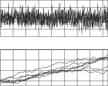
(e)Plot the observation obtained.

(f)Try all possible 2K bit patterns, each time forming a candidate group signal and measuring the Euclidean distance from it to the received observation.

(g)Give out the decision on the bit pattern providing the closest candidate group signal to the observation and check whether all bit decisions are correct.

(h)Run the program, increasing the noise level, and comment on the results.

7.37.Write a program computing total squared correlation and average squared correlation per signature pair for an arbitrary synchronous signature set.

7.38.Write a program constructing an oversaturated binary Welch-bound set of K ¼ 2n signatures of arbitrary length N < K. Use the set obtained in simulating K-user synchronous CDMA. Steps to be done:

(a)Construct a Hadamard matrix of size K.

(b)Discard N K rows in it and use the columns of the truncated matrix as signatures.

(c)Form the K-dimensional vector of users’ data, and use it to manipulate signatures and form a group signal.

(d)Simulate K single-user receivers, each calculating the correlation of the received group signal with an appropriate signature and taking the decision according to the polarity of the correlation.

(e)Compare the K-dimensional vector of decisions on the data with the one really transmitted and find the number of erroneous bits.

(f)Repeat items (c)–(e) 1000–10 000 times and find the bit error probability per user.

(g)Run the program for n ¼ 5, 6, 7, 8 finding each time the minimal length N (maximal oversaturation K/N) where errors do not still occur.

7.39.Write a program simulating an asynchronous CDMA employing time-offset replicas of the same binary m-sequence. Recommended steps:

(a)Set the maximal number of users K ¼ 20 25 and the maximal delay in number of chips mmax ¼ 80 100.

(b)Form the binary f 1g m-sequence of length L K(mmax þ 1).

(c)Take as K signatures K cyclic replicas of the m-sequences, each delayed from the previous by mmax þ 1.

(d)Pick out Ka first signatures (active users) and manipulate all but the first by random independent bits, bit duration fixed within N ¼ 160 200 chips.