


68 |
Spread Spectrum and CDMA |
|
|
2.40.In some system signal duration was quadrupled, signal power remaining unchanged. What happens to the standard deviation of the frequency estimation?
2.41.Horizontal sections of the ambiguity function for four signals are given in Figure 2.36, all sizes marked by the same symbols ( c1 etc.) being equal. Which of the signals is best for:
(a)Measuring only time delay?
(b)Measuring only frequency shift?
(c)Measuring both time delay and frequency shift?
F |
F |
|
F |
|
|
|
F |
|
|
|
|
τc1 |
|
|
|
|
|
Fe1 |
Fe2 |
|
Fe1 |
|
F |
|
|
|
τ |
τ |
τ |
e1 |
τ |
||||
|
|
|
||||||
τc1 |
|
|
Fe2 |
|
|
|
|
|
|
|
|
|
|
|
|
τc2 |
|
|
τc2 |
|
τc2 |
|
|
|
|
|
(a) |
(b) |
|
(c) |
|
|
|
(d) |
|
|
Figure 2.36 Horizontal sections of the ambiguity function |
|
|
|||||
2.42.In the course of modernizing some system operating originally with a plain signal, emitted power was reduced by 6 dB. At the same time signal duration was increased by four times and the plain signal was replaced by a spread spectrum one with time frequency product WT ¼ 100. What happens to the standard deviations of time delay and frequency estimations as compared to the initial ones?
2.43.Which of the signals having the ambiguity diagrams of Figure 2.36 is best for:
(a)Time resolution?
(b)Frequency resolution?
(c)Time–frequency resolution?
2.44.Horizontal sections of the ambiguity function for four signals are given in Figure 2.37, all sizes marked by identical symbols being equal. Which of the signals is best for:
(a)Time resolution?
(b)Frequency resolution?
(c)Time–frequency resolution?
Matlab-based problems
2.45.Write a program illustrating the receiver decision on which of two competitive signals is received. Do the following:

Classical reception problems and signal design |
69 |
F |
F |
Fe |
Fe |
τ |
τ |
τc |
τc |
(a) |
(b) |
F |
F |
Fe |
Fe |
τ |
τ |
τc |
τc |
(c) |
(d) |
Figure 2.37 Horizontal sections of the ambiguity function
(a)Form and plot two 100-dimensional antipodal signal vectors with elements f1g.
(b)Choose one of them as a transmitted signal.
(c)Form the 1000 100 matrix of Gaussian noise, putting standard deviation 6–10 times higher than the square root of the signal energy.
(d)Form the 1000 100 observation matrix, each row being the sum of signal of point (b) and noise; plot observations.
(e)For every observation calculate two distances (or another sufficient statistic) from the observation to each of the two signals.
(f)For every observation take the minimum-distance decision.
(g)Compare the decision with a preset signal of point (b) for each observation.
(h)Calculate the number of errors in all 1000 observations.
(i)Retaining the signal vector lengths and noise deviation, change the signals into an orthogonal pair and run the program again.
(j)Do the same as in (i) for the pair of signals with positive correlation coefficient and for the pair with the second signal equal to zero.
(k)Compare the results of items (i)–(k), both with each other and with theoretical predictions, and give your comments.
2.46.Write a program calculating and plotting binary transmission error probability versus SNR for an arbitrary pair of signals preset as vectors. Use power SNR defined for average energy of the signals:
q2 ¼ E1 þ E2 N0
70 |
Spread Spectrum and CDMA |
|
|
E1, E2 and N0 being the energies of the two signals and the one-sided power spectrum of AWGN. Plot all of the curves in logarithmic scale. Run the program, and compare and explain results for:
(a)Signal pairs of equal energies: antipodal, with negative correlation, orthogonal, with positive correlation.
(b)The pair where one of signals is zero.
2.47.Write a program calculating and plotting (in logarithmic scale) curves of the message recognition error probabilities versus SNR per bit (see Figure 2.9) when m-bit messages are transmitted over an AWGN channel, including for each value of m:
(a)The accurate error probability for bit-by-bit uncoded transmission of M ¼ 2m messages.
(b)The accurate error probability for transmission of M ¼ 2m messages by the orthogonal signals.
(c)The union bound on the error probability for transmission of M ¼ 2m messages by the orthogonal signals.
Run the program for m ¼ 1 to 10 and interpret the behaviour of the curves. Explain why for m ¼ 1, 2 the uncoded transmission curves go lower than the orthogonal signalling ones. For m ¼ 3 to 10, find the values of the orthogonal coding gain corresponding to the error probabilities 10 3, 10 5 and compare them with the asymptotic ones.
2.48.Write a program demonstrating experimentally energy gain of orthogonal coding as compared to uncoded transmission of a 6-bit message. The following operations are relevant:
(a)Form and plot an uncoded 6-bit pattern corresponding to BPSK mode oversampled with Ns samples per bit (it is advisable to take Ns ¼ 64, i.e. 384 samples over 6 bits).
(b)Form the 1000 6Ns matrix of the Gaussian noise samples with standard deviation equal to a quadrupled bit amplitude.
(c)Form and plot the 1000 6Ns matrix of observations, adding the signal to the noise matrix.
(d)Demodulate all observations, calculate and output the message-wise error rate.
(e)Form the Hadamard matrix of order 64, take one of its rows as an encoded message and oversample it into the signal vector of dimension 6Ns.
(f)Repeat items (b)–(d).
(g)Compare and treat the error rates for the two explored transmission modes.
(h)Run the program for the range of SNR, changing the noise level; record the results and compare them with theoretical ones (see Figure 2.9).
2.49.Write a program demonstrating experimentally the trade-off between energy gain and spectral efficiency of the orthogonal signalling. The following operations are relevant:
(a)Set the number of bits m ¼ 8.

Classical reception problems and signal design |
71 |
|
|
(b)Form all possible 2m ¼ 256 bit patterns and oversample them so that each bit occupies 160 samples.
(c)Calculate the power spectra of all bit patterns and the average power spectrum under uncoded transmission.
(d)Form the Hadamard matrix of order 256 and oversample it to come to the same dimension of signal vectors as previously.
(e)Calculate the power spectra of all 256 orthogonal signals and the average power spectrum under orthogonal signalling.
(f)Plot the average power spectra, estimate and compare the bandwidths occupied for both investigated cases and compare their ratio to the theoretical prediction.
2.50.Write and run a program illustrating optimal measurement of the amplitude of the
triangle pulse of duration T: s(t; A) ¼ As(t) ¼ AtT , 0 t T (see Figure 2.38). The following steps should be fulfilled:
Figure 2.38 Simulation of measuring amplitude
(a)Specify the value of amplitude A on your own and form a signal vector of dimension around 100.
(b)Form 10 vectors of the Gaussian noise n(t) with standard deviation approximately equal to the preset signal amplitude.
(c)Form 10 vectors of the observation y(t) by adding noise vectors to the signal vector.

72 |
Spread Spectrum and CDMA |
|
|
(d)Plot waveforms of the observations. Is the signal clearly visible in them?
(e)Calculate and plot the curves of the decision statistics (distances or squared distances or differences Az A2E/2) for all 10 observations versus amplitude estimation.
(f)Find optimal estimations of A for all 10 observations.
(g)Calculate average and variance of the optimal estimations over all observations.
(h)Run the program with several preset values of A and compare the results of measuring with the preset values. Give a theoretical explanation for the results.
2.51. Write and run a program illustrating the optimal measurement of time delay of the bell-shaped baseband pulse of duration T (by the level 0.01). Assume2 [0, 9T]. The following steps illustrated by Figure 2.39 should be completed:
Figure 2.39 Simulation of measuring time delay
(a) Use around 1000 sample points over the whole observation interval2 [0,10T]. Preset the value of (in number of sampling points) on your own and form the time-shifted signal vector;
(b)Form 100 vectors of Gaussian noise n(t) with standard deviation within the range 1 to 2 times the signal amplitude.
(c)Form 100 observation vectors y(t) by adding noise vectors to the signal vector.
(d)Plot waveforms of the observations (see Figure 2.39). Is the signal clearly visible in them?
Classical reception problems and signal design |
73 |
|
|
(e)Calculate and plot curves of the correlations between observations and timeshifted signal copies versus time shift. Is the signal effect now more visible?
(f)Find optimal estimations of for all 100 observations.
(g)Calculate the average and the variance of optimal estimations over all observations.
(h)Run the program with several preset values of and in the range of SNR. Compare the results of measurements with the preset values. Give a theoretical explanation for the results.
2.52.The bandpass rectangular pulse of duration T is applied to a bandpass filter with rectangular pulse response of duration 2T, which is frequency-detuned against the signal by F. Based on the complex envelope, calculate and plot signal shapes (real envelopes) at the filter output for F ¼ a/T, where a ¼ 0, 0:5, 1:0.
2.53.The bandpass rectangular pulse of duration T and carrier frequency f0 ¼ 10/T is applied to the bandpass filter with rectangular pulse response of the same duration
which is frequency-detuned against the signal by F 2 f0, T1 , T2 g. Based on the complex envelope, calculate and plot the bandpass signals at the filter output for all three values of F.
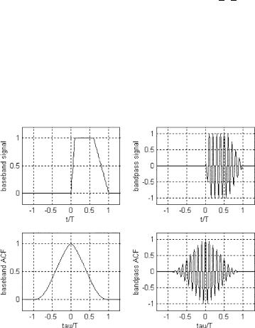
2.54.Write a program calculating and plotting the autocorrelation function of both baseband and bandpass signals of the same arbitrary form and duration T. Take the carrier frequency of the baseband signal equal to 10/T. See the example in Figure 2.40. Run the program for:
(a)Rectangular pulse.
(b)Triangular symmetric pulse.
Figure 2.40 Autocorrelation functions of baseband and bandpass signals
74 |
Spread Spectrum and CDMA |
|
|
(c) Triangular pulse rising within [0, T).
(d)Pulse of your own choice.
2.55.Write a program demonstrating the time-compression effect in a matched filter. Take a rectangular linearly-frequency-modulated (LFM) signal of duration T with complex envelope:
S_ t |
8 exp j |
Td |
|
; 0 t T |
||
ð Þ ¼ |
> |
|
|
W t2 |
|
|
|
< |
0; t < 0 or t > T |
||||
|
> |
|
|
|
|
|
|
: |
|
|
|
|
|
Take the initial carrier frequency f0 ¼ 50/T and five values of frequency deviation Wd ¼ a/T, a 2 f0, 10, 20, 30, 40g. For each value of deviation show bandpass signals at the matched filter input and output.
2.56.Write a program illustrating the dependence of the accuracy of time-delay estimation on the signal bandwidth (see Figure 2.21). Take an LFM signal with the bellshaped envelope, i.e. the complex envelope:
|
S_ t |
8 exp" 20 T |
2 |
# exp j |
Td |
|
; 0 t T |
|
|
||||||
|
ð Þ ¼ |
> |
|
t |
1 |
|
2 |
|
|
W |
t2 |
|
|
|
|
|
|
> |
|
|
|
|
|
|
|
|
|
|
|
|
|
|
|
< |
|
|
|
|
|
|
|
|
|
|
|
|
|
|
|
> |
0; t < 0 or t > T |
|
|
|
|
|
|
|
|
|
|||
|
|
> |
|
|
|
|
|
|
|
|
|
|
|
|
|
Perform |
|
: |
|
|
|
|
|
|
|
|
|
of the deviation W |
d ¼ |
a/T, |
|
|
calculation and plotting |
for the |
values |
|
|||||||||||
|
|
|
|||||||||||||
a ¼ 0, 10, 25, 50. The following steps should be completed:
(a)Specify the value of the deviation Wd and form the signal (complex envelope) vector of dimension around 100.
(b)Plot the real envelope of the signal.
(c)Form 100 vectors of the complex Gaussian noise with standard deviations of real and imaginary parts within [0.5, 4.0].
(d)Form 100 observation vectors by adding noise vectors to the signal vector.
(e)Plot waveforms of the real envelopes of the observations. Is the signal clearly visible in them?
(f)Calculate and plot curves of the matched filter output real envelopes for all 100 observations.
(g)Find the time positions of the maximums of matched filter output real envelope for all 100 observations.
(h)Calculate the average and the variance of the time-delay estimations over all 100 observations.
(i)Compare data for different Wd and treat the results theoretically.
2.57.Write a program demonstrating resolution of two time-shifted bandpass rectangular pulses of duration T. Take the signal of Problem 2.55 with the same values of carrier frequency and deviation (Figure 2.27). Recommended steps:
(a)Specify the value of the deviation Wd and form the signal (complex envelope) vector of necessary dimension.

Classical reception problems and signal design |
75 |
|
|
(b)Form and plot a bandpass signal.
(c)Specify the value of delay 0 < < T, form and plot a delayed signal copy.
(d)Calculate and plot superposition of the two signals.
(e)Calculate and plot matched filter response to it.
(f)Run the program, varying the frequency deviation and delay, and give a theoretical treatment of the results.
2.58.Write a program calculating and plotting the time–frequency ambiguity function of a plain bandpass pulse with arbitrary real envelope and duration T. Provide for plotting also the basic sections of the ambiguity function (along the and F axes) as well as the horizontal section at the level 0.5. Run the program for:
Figure 2.41 Ambiguity function of a rectangular pulse
(a)Rectangular pulse (see Figure 2.41).
(b)Triangular symmetric pulse.
(c)Triangular pulse rising within [0,T).
(d)Pulse of your own choice.