


62 |
|
Spread Spectrum and CDMA |
Table 2.1 Role of spread spectrum signals in the classical reception problems |
||
|
|
|
Problem |
Performance-influencing |
Spread spectrum signals |
|
signal parameters |
|
|
|
|
Detection, amplitude |
SNR (signal energy only) |
Unnecessary |
and phase measurement |
|
|
Binary data |
SNR, correlation coefficient |
Unnecessary |
transmission (M ¼ 2) |
|
|
M-ary data |
SNR, correlation |
Unnecessary but |
transmission, M > 2 |
coefficients of all signals |
sometimes attractive from |
|
|
an implementation |
|
|
standpoint |
Time delay measurement, |
SNR, signal bandwidth |
Unnecessary when |
time-resolution |
|
power-limit-free, |
|
|
necessary otherwise |
Frequency measurement, |
SNR, signal duration |
Unnecessary |
frequency resolution |
|
|
Time–frequency |
SNR, signal bandwidth and |
Necessary |
measurement, |
duration |
|
time–frequency resolution |
|
|
|
|
|
seem very odd and lead to questioning of the grounds for the wide popularity of spread spectrum nowadays. As the following chapter shows, however, these grounds are quite solid and manifest themselves clearly whenever we base our study on a more realistic channel model than the sometimes ‘academic’ Gaussian one, or need to draw in some additional performance criteria.
Problems
2.1.Three signals s1(t), s2(t), s3(t) are given in Figure 2.28.
By how many times is the maximum distance in this signal set greater than the minimum one?
 s1(t)
s1(t)
U
T t
s2(t)
T/2 |
t |
–2U
2U
s3(t)
t
Figure 2.28 Set of three signals

Classical reception problems and signal design |
63 |
|
|
2.2.Observation y(t) at the AWGN channel output is given in Figure 2.29, and the input signals are the same as in Problem 2.1. What will the decision of the optimal receiver be?
y(t)
U
T/2
T t
–U
Figure 2.29 Waveform at the channel output
2.3.A source generates data at the rate R ¼ 10 kbps. Each bit of the source data is transmitted over the AWGN channel by BPSK. Bandwidth W ¼ 10 MHz is available in principle. Is it reasonable to use signals with bandwidth W ¼ 10 MHz?
2.4.What is better for BPSK signalling over a Gaussian channel?
(a)Rectangular pulses of peak power 1000 W with bandwidth 100 kHz.
(b)Rectangular pulses of the same duration with peak power 900 W and bandwidth 10 MHz?
2.5.Calculate the energy losses for the pairs of signals of Figure 2.30 used for binary transmission over the AWGN channel with respect to the optimal pair.
U |
|
|
|
|
U |
|
|
|
|
t |
U |
|
|
|
|
t |
|
|
|
|
|
|
|
|
|
|
|
|
|||||
|
|
|
|
|
|
|
|
|
|
|
|
|
|
|||
|
|
|
T |
t |
|
|
|
|
T |
–U |
|
|
|
T |
||
U |
|
|
|
|
U |
|
|
|
|
|
|
|
|
|
||
|
|
|
|
|
|
|
|
U |
|
|
|
|
|
|||
|
|
|
|
t |
|
|
|
|
|
t |
|
|
|
|
|
t |
–U |
2T/3 |
|
|
–U T/3 |
|
|
–U |
|
T/3 |
|
|
|||||
|
|
|
|
|
|
|
|
|
|
|||||||
(a) |
|
|
(b) |
|
|
(c) |
||||||||||
|
|
|
|
|
|
|
|
|
||||||||
|
|
|
|
|
|
|
|
|
||||||||
Figure 2.30 Three signal pairs
2.6.In differential BPSK (DBPSK) a bit content is transmitted by alternation or nonalternation of the polarities of two consecutive pulses, identical polarities corresponding to zero and different polarities to one. Compare to the first approximation DBPSK and BPSK in energy consumption (based on minimum distances only) and the bandwidth occupied, transmission rates being the same.
2.7.In quadrature PSK (4-PSK or QPSK) two bits (four messages) are transmitted by
four signal phases: 0, , /2. Is this an optimal transmission mode for two bits? If not, describe a better technique and its asymptotic coding gain against QPSK.
2.8.Is it possible to have 10 equidistant signals with correlation coefficient between any two of them equal to 1/7? What is the maximal possible number of signals with this correlation coefficient?
64 |
Spread Spectrum and CDMA |
|
|
2.9.Calculate and sketch versus M the energy loss (in dB) of the set of M orthogonal signals as compared to the set of M optimal signals (AWGN channel). Find the asymptotic loss when M grows.
2.10.Asymptotic energy gain of orthogonal coding against uncoded binary transmission for the case of M ¼ 2 messages turns to be 1/2 or 3 dB, i.e. negative, showing loss rather than gain. What does this mean physically?
2.11.Asymptotic energy gain of orthogonal coding against uncoded binary transmission for the case of M ¼ 4 messages turns to be 1 (0 dB), i.e. no gain at all. Give the physical reasoning for the result.
2.12. In 8-PSK M ¼ 8 messages are transmitted by identical bandpass pulses having 8 different equidistant initial phases. Is this way of transmitting 8 messages over the Gaussian channel the best possible one if no bandwidth limitation is imposed? If not, what is the energy loss of 8-PSK against the optimal set of M signals?
2.13.Compare asymptotic (determined by minimum distance) efficiency of M-PSK against orthogonal coding in energy consumption (given the error probability) and bandwidth occupied.
2.14.In the IS-95 mobile phone uplink blocks of 6 bits are transmitted by orthogonal signals. The transmission rate is 28.8 kbps. Estimate the bandwidth occupied by the encoded signals (ignoring further spreading by the long code).
2.15.In a digital communication system the allowed bandwidth W ¼ 1:2288 MHz. What maximal number of orthogonal signals M may be used for data transmission at the rate of 38.4 kbps?
2.16.In a system data is transmitted over the Gaussian channel at the rate of 10 kbps. The system designer tries to provide 6 dB energy gain against the uncoded transmission. Is this achievable on the basis of orthogonal signals if only bandwidth within 320 kHz is tolerable?
2.17.Some system is allowed to use bandwidth of 10.24 MHz while the necessary transmission rate is 100 kbps. What potential asymptotic coding gain is achievable in the system?
2.18.It is necessary to transmit data over the Gaussian channel at the rate of 100 kbps using carrier frequency 2 GHz. Is it realistic to count on energy gain G ¼ 10 dB on the basis of orthogonal signals?
2.19.Build up the Hadamard matrix of size 16.
2.20.Which of the following transformations preserve/violate the main property (orthogonality of rows) of a Hadamard matrix?
(a)Permutation of rows.
(b)Permutation of columns.
(c)Simultaneous alternation of signs of all elements.
(d)Alternation of signs of all elements of several rows.
(e)Alternation of signs of all elements of several columns.
(f)Alternation of sign of upper leftmost element only.
2.21.Hadamard matrix HM of size M ¼ 2m is built up by the Sylvester rule starting with
H2 ¼ |
1 |
1 |
. The first column of HM is discarded and the rows of the matrix |
1 |
1 |
thus obtained are used to generate signals for M-ary transmission. What sort of
Classical reception problems and signal design |
65 |
|
|
signal ensemble do we have this way? What is the bandwidth they occupy in comparison with orthogonal ones?
2.22. LFM signal (with linear frequency modulation):
s t |
Þ ¼ |
8 A cos 2 f0t þ Wd ðT Þ |
|
þ ; jt j T=2 |
||
ð |
> |
" |
|
# |
||
|
|
|
|
t |
2 |
|
|
|
> |
|
|
|
|
|
|
< |
|
|
|
|
|
|
> |
0; jt j > T=2 |
|
|
|
|
|
> |
|
|
|
|
|
|
: |
|
|
|
|
has amplitude A, carrier frequency f0, frequency deviation Wd , duration T, time delay and initial phase ’. Classify these six parameters as energy or non-energy ones. (For any bandpass signal f0T 1, W f0.)
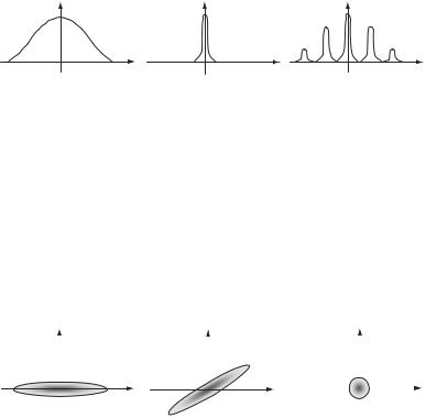
2.23.Non-energy signal parameter needs to be measured. The correlation coefficient( ) of the signal copies detuned in is shown in Figure 2.31 for three different cases. In which of these will the accuracy of measuring be highest?
ρ(λ) |
ρ(λ) |
ρ(λ) |
λ |
λ |
λ |
(a) |
(b) |
(c) |
Figure 2.31 Dependence of correlation coefficient on a measured parameter
2.24.Two non-energy scalar parameters 1, 2 need to be measured simultaneously. The correlation coefficient of two signal copies with different pairs of values of1, 2 is ( 1, 2) and geometrically is represented by some surface in threedimensional space. A cross-section of this surface by a horizontal plane at some level (e.g. 0.5) is given in Figure 2.32 for three typical cases. In which of these will the accuracy of simultaneous estimation of 1, 2 be highest if no a priori knowledge about their values is available?
λ2 |
|
λ1 |
λ2 |
|
λ1 |
λ2 |
|
|
λ1 |
|
|
|
|||||||
|
|
|
|
|
|
|
|||
|
|
|
|
|
|
|
|||
|
|
|
|
|
|
|
|
|
|
(a) |
(b) |
(c) |
|||||||
Figure 2.32 Horizontal sections of the surface ( 1, 2)
66 |
Spread Spectrum and CDMA |
|
|
2.25.Amplitude A of the signal s(t; A) ¼ As(t) needs to be measured. The reference signal s(t) for three cases is given in Figure 2.33. In which of these cases will the accuracy of measuring A be highest?
U |
s(t) |
|
U |
s(t) |
|
U/ 2 |
s(t) |
|
|
|
|
|
|
|
|||
|
|
|
|
T/2 |
T |
|
|
|
–T/2 |
0 T/2 |
t |
–T |
0 |
t |
–T |
0 |
T t |
|
|
|
|
–U |
|
|
|
|
(a) |
(b) |
(c) |
Figure 2.33 Three forms of a reference signal
2.26. Amplitude A of the signal s(t; A) ¼ As(t) is measured. Someone is dissatisfied with the accuracy of the amplitude estimation. How many times should the duration of the reference signal s(t) be increased in order to halve the standard deviation of the estimation of A, all the other parameters of s(t) remaining the same?
2.27. Amplitude A of the signal s(t; A) ¼ As(t) is measured. The amplitude of the reference signal s(t) is doubled while its duration is halved. What happens to the standard deviation of the estimation of A?
2.28. The initial phase of the bandpass signal needs to be measured. What happens to the standard deviation of the phase estimation when:
(a) Carrier frequency of the signal is doubled?
(b) Signal duration is doubled?
(c) Signal amplitude is halved?
(d) Signal amplitude is doubled and duration is reduced by four times?
2.29. The initial phase of the bandpass signal needs to be measured. Three variants of the signal envelope are given in Figure 2.33. In which of these cases will the accuracy of phase measurement be highest?
2.30. The initial phase ’ of the LFM signal of Problem 2.22 is measured. Variation of which of the parameters A, f0, Wd , T, and in which direction will affect the
precision of the phase estimation? What happens to the standard deviation of p
the phase estimation when A, f0, Wd are all increased by 2 times while T and are halved?
2.31.Sketch the autocorrelation functions of the three signals shown in Figure 2.34.
2.32.The bandpass BPSK signal consists of three consecutive rectangular pulses each being of duration D. The phases of the first two equal zero while the third phase is . Sketch the autocorrelation function of the signal.
2.33.The matched filter for a rectangular baseband pulse of duration D is given. What sort of circuitry should be added to it in order to obtain the matched filter for the signals of Figure 2.34? Sketch the response of the filter matched to signal (c) when this very signal inputs the filter.

Classical reception problems and signal design |
|
|
|
|
67 |
||||||||||
|
|
|
|
|
|
|
|
|
|
|
|
|
|
|
|
|
U |
|
|
s(t) |
|
|
U |
s(t) |
|
|
U |
s(t) |
|
|
|
|
|
|
|
|
|
|
|
t |
|
|
|
|
|||
|
|
|
|
|
|
|
|
|
|
|
|||||
|
|
|
|
|
|
|
|
|
|
|
|
|
|
|
|
|
–∆ |
|
0 |
∆ |
t |
|
0 ∆ 2∆ |
3∆ |
|
0 ∆ 2∆ |
3∆ |
4∆ |
t |
||
|
|
|
–U |
|
|
|
|
–U |
|
|
|
–U |
|
|
|
|
|
|
|
|
|
|
|
|
|
|
|
|
|
|
|
|
|
|
(a) |
|
|
|
(b) |
|
|
|
(c) |
|
|
|
|
Figure 2.34 Three forms of a signal
2.34.The matched filter for a rectangular bandpass pulse of duration D is given. What circuitry added to it will produce a matched filter for the signal of Problem 2.32? Sketch the response of the matched filter to the signal of Problem 2.32.
2.35.The autocorrelation functions of three alternative signals are given in Figure 2.35. Which of these is best for measuring time delay?
ρ(τ) |
|
(a) |
|
ρ(τ) |
τ |
(b) |
|
ρ(τ) |
τ |
|
|
(c) |
|
|
τ |
Figure 2.35 Examples of autocorrelation function
2.36. Parameters of the plain pulse signal provide standard deviation of time-delay
|
m |
|
¼ p |
¼ |
|
measurement 0:5 |
|
s and SNR at the matched filter output q |
2E/N0 |
|
10. |
Estimate roughly the signal duration.
2.37.In some radar a plain pulse signal is used. The system designer wants to reduce the peak-power by 100 times without sacrificing SNR and at the same time to reduce by 10 times the standard deviation of measuring time delay. What should the time–frequency product of the signal in the improved radar be?
2.38.In some radar distance is measured through emitting LFM pulse (see Problem 2.22) with time–frequency product WT ¼ 103. Due to a breakage of the modulator the radar started emitting unmodulated pulses of the same peak-power and duration. What happens to the standard deviation of distance measuring?
2.39.In some system it is necessary to reduce by 10 times the standard deviation of frequency measurement. The signal power can be increased only 25/16 times (1.94 dB). How should the signal duration be changed?