

Литература / Handbook of Applied Cryptography / chap6
.pdf200 |
Ch. 6 Stream Ciphers |
ìMLON |
|
|
|
|
ôJI ô K |
|
|
ë )SRQ»line |
|
|
|
|
|
|
20 |
|
|
|
|
15 |
|
|
|
|
10 |
|
|
|
|
5 |
|
|
|
|
10 |
20 |
30 |
40 |
P |
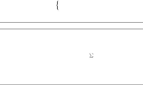
Figure 6.6: Linear complexity profile of the TVU-periodic sequence of Example 6.26.
As is the case with all statistical tests for randomness (cf. ¨5.4), the condition that a sequence èhave a linear complexity profile that closely resembles that of a random sequence is necessary but not sufficient for èto be considered random. This point is illustrated in the following example.
6.27Example (limitations of the linear complexity profile) The linear complexity profile of the sequence èdefined as
®° µ ¶if ´°D·éæ µfor some ªÇ, |
|
è |
Ç ¶otherwise¶ |
|
|
follows the line å ° ( ·Aas closely as possible. That is, å(Á¯è°-XW)ÁÂ?(úDµÂ?A·VYfor all ( ªµ. However, the sequence èis clearly non-random.
6.2.3 Berlekamp-Massey algorithm
The Berlekamp-Massey algorithm (Algorithm 6.30) is an efficient algorithm for determining the linear complexity of a finite binary sequence è-+of length ©(see Definition 6.18). The algorithm takes ©iterations, with the (th iteration computing the linear complexity of the subsequence è-)consisting of the first ( terms of è-.+The theoretical basis for the algorithm is Fact 6.29.
6.28 Definition Consider theëfinite binary sequence è)ͺ° èÔK¶èº ¶U¹è)¹U¹ê¶áè). For ¾sÁ÷ö  °Dµ ºúö ú ûUû öû¯ú, letõ1å¯ë¶¾sÁ¯öbe an LFSR that generates the subsequence è-)° èԶ躶U¹ è¹U¹ê¶áº. The next discrepancy Z) is the difference between è) and the Á?(úFµÂ\[7] term generated) by the LFSR: Z) ° Á¯è) ú ®ë^Qºè®)á9®Â ·. _
6.29 Fact Let è-)° èԶ躶 ¹ è¹U¹ê¶)áºbe a finite binary sequence of linear complexity å ° å(Á¯è)Â, and let õ ¶å¾sÁ¯öbe an LFSR which generates è).
Êc 1997 by CRC Press, Inc. — See accompanying notice at front of chapter.
Ë6.2 Feedback shift registers |
201 |
(i)The LFSR õ ¶å¾sÁ÷öalsoÂ÷øgenerates è,)ͺ° èÔ趺 ¶ ¹è)¹U¹f¶áè) if and only if the
next discrepancy Z) is equal to 0.
(ii)If Z) °|Ç, then å(Á÷è)ͺ° å.
(iii)Suppose Z) ° .µLet ± the largest integer G ( such that åAÁ¯èÜÂG å(Á¯è, and-) letÂ
õ1åAÁ¯èܶ0 Á¯öbe an LFSR of length е(БчиЬВwhich generates èÜ. Then õ 嶾a`b`ÎÁ¯ö is an LFSR of smallest length which generates è-Í)º, where
° å¶ |
if åc@#(·, A |
|
å` |
( ú æµ ¶å if åç ( ·A, |
|
|
||
and ¾b`ÎÁ¯öh°¾sÁ÷öú0ÂÁ¯öhÂûd)áÜ.
6.30Algorithm Berlekamp-Massey algorithm
INPUT: a binary sequence è-+° èÔK¶èºè¶»K¶ ¹U¹è+ẹf¶of length ©. OUTPUT: the linear complexity åAÁ¯è+Âof è+, Ç%çå(Á÷è+Âç©.
1.Initialization. ¾sÁ¯öµ, Âå,eeÇ, ±e æµ, 0 Á¯öµ, Â(fe,eÇ.
2.While Á?(G ©(Âdo the following:
2.1Compute the next discrepancy Z. Z e7Á÷è) ú ®ëgQºè®)á<®Â ·.
2.2If Z° thenµ do the following:
hÁ¯ö Â,e~, ¾sÁ÷ö  eú 0¾sÁ¯Á¯öû hÂd)ÂáÜ.
If åç ( ·Athen å ei(ú æ~åµ, ± e=(, 0 Á¯öhÂÁ¯öhÂe.
2.3(fei(ú .µ
3.Return(å).
6.31Note (intermediate results in Berlekamp-Massey algorithm) At the end of each iteration of step 2, õ1嶾sÁ¯öhÂ÷øis an LFSR of smallest length which generates è,). Hence, Algorithm 6.30 can also be used to compute the linear complexity profile (Definition 6.23) of a finite sequence.
6.32Fact The running time of the Berlekamp-Massey algorithm (Algorithm 6.30) for determining the linear complexity of a binary sequence of bitlength ©is jsÁ©»Âbit operations.
6.33Example (Berlekamp-Massey algorithm) Table 6.1 shows the steps of Algorithm 6.30 for
computing the linear complexity of the binary sequence è,+° Ç ¶ ÇK¶ µK¶ ofµlength¶ Ç ¶ µ ¶ µK¶ µK¶ Ç
©° . This sequence is found to have linear complexity and an LFSR which generates
it is õ¶ µ&úö¼ú ö4ø. |
|
6.34 Fact Let è-be+ a finite binary sequence of length ©, and let the linear complexity of è-be+ å. Then there is a unique LFSR of length åwhich generates è-+if and only if åç +».
An important consequence of Fact 6.34 and Fact 6.24(iii) is the following.
6.35Fact Let èbe an (infinite) binary sequence of linear complexity å, and let äbe a (finite) subsequence of èof length at least ·å. Then the Berlekamp-Massey algorithm (with step 3 modified to return both åand ¾sÁ÷ö) on input ädetermines an LFSR of length åwhich generates è.
Handbook of Applied Cryptography by A. Menezes, P. van Oorschot and S. Vanstone.
202 |
|
|
|
|
|
|
|
|
|
|
|
|
|
|
|
|
|
|
|
|
|
|
|
|
Ch. 6 Stream Ciphers |
||||
|
|
|
|
|
|
|
|
|
|
|
|
|
|
|
|
|
|||||||||||||
|
|
è |
|
Z |
|
hÁ÷ö  |
|
|
¾sÁ¯ö  |
|
å |
|
± |
|
0 Á¯öh |
|
( |
|
|||||||||||
|
|
|
|
|
|
|
|
|
|
||||||||||||||||||||
|
|
|
|
|
|
|
|
|
|
|
|||||||||||||||||||
|
|
) |
|
æ |
|
æ |
|
|
|
|
|
|
µ |
|
|
|
|
|
Ç |
|
æµ |
|
µ |
|
|
Ç |
|
||
|
|
æ |
|
|
|
|
|
|
|
|
|
|
|
|
|
|
|
|
|
|
|||||||||
|
|
Ç |
|
Ç |
|
æ |
|
|
|
|
|
|
µ |
|
|
|
|
|
Ç |
|
æµ |
|
µ |
|
|
µ |
|
||
|
|
Ç |
|
Ç |
|
æ |
|
|
|
|
|
|
µ |
|
|
|
|
|
Ç |
|
æµ |
|
µ |
|
|
· |
|
||
|
|
µ |
|
µ |
|
µ |
|
|
|
|
|
µ?ú ¼ |
|
|
|
|
¸ |
|
· |
|
µ |
|
|
¸ |
|
||||
|
|
µ |
|
µ |
µ?ú |
¼ |
|
|
|
|
|
ö |
|
¼ |
|
|
¸ |
|
· |
|
µ |
|
|
|
|
||||
|
|
|
|
|
|
µ?ú ú |
|
|
|
|
|
|
|
¬ |
|
||||||||||||||
|
|
|
|
|
|
|
ö |
|
¼ |
|
|
ö |
|
ö |
|
¼ |
|
|
|
|
|
|
|
|
|
||||
|
|
Ç |
|
µ |
µ?ú ú |
|
|
µ?ú ú |
» |
|
|
|
¸ |
|
· |
|
µ |
|
|
|
|
||||||||
|
|
|
|
|
|
¼ |
ö |
ú |
|
|
|
|
|
|
|
|
|
||||||||||||
|
|
µ |
|
µ |
|
ö |
|
»ö |
|
ö |
|
|
»ö |
|
¸ |
|
· |
|
µ |
|
|
|
|
||||||
|
|
|
µ?ú ú |
ö |
|
ú |
ö |
|
µ?ú ú |
ö |
|
|
|
|
|
|
|
« |
|
||||||||||
|
|
|
|
|
ö |
|
» |
|
¼ |
|
ö |
|
|
|
|
|
|
|
|
|
|
|
|
||||||
|
|
µ |
|
Ç |
µ?ú ú |
|
|
|
µ?ú ú |
|
» |
|
|
¸ |
|
· |
|
µ |
|
|
|
|
|||||||
|
|
|
ö |
|
ú |
ö |
|
ö |
|
|
|
|
|
|
|
|
|
||||||||||||
|
|
µ |
|
µ |
ö |
|
|
|
|
|
|
ö |
|
|
4 |
|
|
|
|
|
µ?ú ú |
» |
|
|
|
||||
|
|
|
µ?ú ú |
|
» |
|
µ?ú ú |
»ú |
|
|
|
|
|
|
|||||||||||||||
|
|
|
|
|
|
ö |
|
|
ö |
|
|
ö |
|
ö |
|
|
ö |
|
|
|
|
|
ö |
ö |
|
|
|
||
Ç |
µ |
µ?ú ú |
ö |
»ú |
ö |
4 |
µ?ú ¼ú |
|
4 |
|
|
|
µ?ú ú |
» |
|
|
|||||||||||||
|
|
|
|
|
ö |
|
|
|
|
|
|
ö |
|
ö |
|
|
|
|
|
|
ö |
ö |
|
|
|
||||
Table 6.1: Steps of the Berlekamp-Massey algorithm of Example 6.33.
6.2.4 Nonlinear feedback shift registers
This subsection summarizes selected results about nonlinear feedback shift registers. A function with ©binary inputs and one binary output is called a Boolean function of ©variables; there are ·»+different Boolean functions of ©variables.
6.36Definition A (general) feedback shift register (FSR) of length åconsists of åstages (or delay elements) numbered Ç ¶ µ å¶ ¹U¹æ, each¹ capable¶ of storing one bit and having one input and one output, and a clock which controls the movement of data. During each unit of time the following operations are performed:
(i) |
the content of stage Çis output and forms part of the output sequence; |
(ii) |
the content of stage ´is moved to stage ´ æµfor each ´, µ ç´ç åwæµ; and |
(iii)the new content of stage å7æµis the feedback bit è¦é° Á÷è¦éÏẶè¦éỶ ¹U¹è¦éá<ë¹ê¶Â,
where the feedback function Ïis a Boolean function and è¦éá9®is the previous content
of stage åwæw´, µ ç´ç å.
If the initial content of stage ´is è®ücÇK¶forµeach Ç ç´ç åsæµ, then þèë3Ạ¶U¹è¹èÔ¹ê¶ÿ is called the initial state of the FSR.
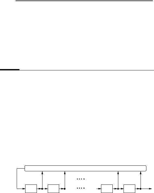
Figure 6.7 depicts an FSR. Note that if the feedback function Ïis a linear function, then the FSR is an LFSR (Definition 6.7). Otherwise, the FSR is called a nonlinear FSR.
|
|
l |
|
|
|
|
|
|
ìí¯óQðìí¯ó9ï ìí¯ó<òN |
|
|
||
ìí |
ìí¯óQð |
ìí¯ó9ïK |
§§÷§m |
ìí¯ó<ò<k ðìí¯ó<ò |
|
|
|
Stage |
Stage |
|
Stage |
Stage |
|
|
L-1 |
L-2 |
|
1 |
0 |
output |
Figure 6.7: A feedback shift register (FSR) of length ô.
6.37Fact If the initial state of the FSR in Figure 6.7 is þèëRẠ¶U¹èº¹U¹ê¶è¶Ôÿ, then the output sequence è° èÔK¶èºè¶»K¶U¹is uniquely¹ ¹ determined by the following recursion:
è¦é°IÏÁ¯è¦éẶèéỶU¹ è¦é¹á9ë¹3¶Âfor ªDå¹
Êc 1997 by CRC Press, Inc. — See accompanying notice at front of chapter.
Ë6.3 Stream ciphers based on LFSRs |
203 |
6.38Definition An FSR is said to be non-singular if and only if every output sequence of the FSR (i.e., for all possible initial states) is periodic.
6.39Fact An FSR with feedback function ÏÁ¯èéáºU¶èéá» ¶ ¹U¹èéá<ë¹ê¶is non-singular if and only
if Ïis of the form ПF°ийб9л²wСБчийбºи¶йб» ¶ ¹ийб9л3Н¹U¹к¶ºВfor some Boolean function Ñ.
The period of the output sequence of a non-singular FSR of length åis at most ·ë.
6.40Definition If the period of the output sequence (for any initial state) of a non-singular FSR of length åis ·ë, then the FSR is called a de Bruijn FSR, and the output sequence is called a de Bruijn sequence.
6.41Example (de Bruijn sequence) Consider the FSR of length ¸with nonlinear feedback function ÏÁ7nºn¶»K¶n¼Â°|µK²n» n²¼ n²ºn». The following tables show the contents of the
¸stages of the FSR at the end of each unit of time äwhen the initial state is þÇ ¶ ÿÇ. ¶ Ç
ä |
Stage 2 |
Stage 1 |
Stage 0 |
|
ä |
Stage 2 |
Stage 1 |
Stage 0 |
|
|
|
|
|
|
|
|
|
Ç |
Ç |
Ç |
Ç |
|
¬ |
Ç |
µ |
µ |
µ |
µ |
Ç |
Ç |
|
|
µ |
Ç |
µ |
· |
µ |
µ |
Ç |
|
« |
Ç |
µ |
Ç |
¸ |
µ |
µ |
µ |
|
Ç |
Ç |
µ |
|
The output sequence is the de Bruijn sequence with cycle Ç ¶ Ç ¶ Ç ¶. µK¶ µK¶ µ ¶ Ç ¶ µ
Fact 6.42 demonstrates that the output sequence of de Bruijn FSRs have good statistical properties (compare with Fact 6.14(i)).
6.42Fact (statistical properties of de Bruijn sequences) Let èbe a de Bruijn sequence that is generated by a de Bruijn FSR of length å. Let ³be an integer, µ çD³å, andç let èbe any subsequenceë3áØ of èof length ·ëú|³æ µ. Then each sequence of length ³appears exactly · times as a subsequence of è. In other words, the distribution of patterns having fixed length of at most åis uniform.
6.43Note (converting a maximum-length LFSR to a de Bruijn FSR) Let oºbe a maximumlength LFSR of length åwith (linear) feedback function ÏÁ¯èéáºè¶éá» ¶U¹èéá9ë¹Â¹3¶. Then
the FSR o»with feedback function ÑÁ¯è¦éẶè¦éỶ ¹U¹è¦éá9ë¹f¶Â°IÏ^²è¦éáºèéá»û ûUûè¦éá9ë3ͺ
is a de Bruijn FSR. Here, è®denotes the complement of è®. The output sequence of o»is obtained from that of oºby simply adding a Çto the end of each subsequence of åZæµ ’sÇ occurring in the output sequence of oº.
6.3Stream ciphers based on LFSRs
As mentioned in the beginning of ¨6.2.1, linear feedback shift registers are widely used in keystream generators because they are well-suited for hardware implementation, produce sequences having large periods and good statistical properties, and are readily analyzed using algebraic techniques. Unfortunately, the output sequences of LFSRs are also easily predictable, as the following argument shows. Suppose that the output sequence èof an LFSR has linear complexity å. The connection polynomial ¾sÁ÷öof anÂLFSR of length åwhich generates ècan be efficiently determined using the Berlekamp-Massey algorithm
Handbook of Applied Cryptography by A. Menezes, P. van Oorschot and S. Vanstone.
204 |
Ch. 6 Stream Ciphers |
(Algorithm 6.30) from any (short) subsequence äof èhaving length at least © ° å·(cf. Fact 6.35). Having determined ¾sÁ÷ö, the ÂLFSR õ1嶾sÁ¯öhÂ÷øcan then be initialized with any substring of ähaving length å, and used to generate the remainder of the sequence è. An adversary may obtain the required subsequence äof èby mounting a known or chosenplaintext attack (¨1.13.1) on the stream cipher: if the adversary knows the plaintext subsequence ±º¶ ±»¶U¹ ¹+¹ê¶1±corresponding to a ciphertext sequence º¶U»¶U¹ ¹+, ¹ê¶Uthe corre - sponding keystream bits are obtained as ± ®÷², µ ç´®ç©.
6.44Note (use of LFSRs in keystream generators) Since a well-designed system should be secure against known-plaintext attacks, an LFSR should never be used by itself as a keystream generator. Nevertheless, LFSRs are desirable because of their very low implementation costs. Three general methodologies for destroying the linearity properties of LFSRs are discussed in this section:
(i)using a nonlinear combining function on the outputs of several LFSRs (¨6.3.1);
(ii)using a nonlinear filtering function on the contents of a single LFSR (¨6.3.2); and
(iii)using the output of one (or more) LFSRs to control the clock of one (or more) other LFSRs (¨6.3.3).
Desirable properties of LFSR-based keystream generators
For essentially all possible secret keys, the output sequence of an LFSR-based keystream generator should have the following properties:
1.large period;
2.large linear complexity; and
3.good statistical properties (e.g., as described in Fact 6.14).
It is emphasized that these properties are only necessary conditions for a keystream generator to be considered cryptographically secure. Since mathematical proofs of security of such generators are not known, such generators can only be deemed computationally secure (¨1.13.3(iv)) after having withstood sufficient public scrutiny.
6.45Note (connection polynomial) Since a desirable property of a keystream generator is that its output sequences have large periods, component LFSRs should always be chosen to be
maximumý -length LFSRs, i.e., the LFSRs should be of the form õ ¶å¾sÁ÷öwhereÂ÷ø¾sÁ÷öü Â
»þö isÿa primitive polynomial of degree å(see Definition 6.13 and Fact 6.12(ii)).
6.46Note (known vs. secret connection polynomial) The LFSRs in an LFSR-based keystream generator may have known or secret connection polynomials. For known connections, the secret key generally consists of the initial contents of the component LFSRs. For secret connections, the secret key for the keystream generator generally consists of both the initial contents and the connections.
For LFSRs of length åwith secret connections, the connection polynomials should be selected uniformly at random from the set of all primitive polynomials of degree åover ý». Secret connections are generally recommended over known connections as the former are more resistant to certain attacks which use precomputation for analyzing the particular connection, and because the former are more amenable to statistical analysis. Secret connection LFSRs have the drawback of requiring extra circuitry to implement in hardware. However, because of the extra security possible with secret connections, this cost may sometimes be compensated for by choosing shorter LFSRs.
Êc 1997 by CRC Press, Inc. — See accompanying notice at front of chapter.
Ë6.3 Stream ciphers based on LFSRs |
205 |
6.47Note (sparse vs. dense connection polynomial) For implementation purposes, it is advantageous to choose an LFSR that is sparse; i.e., only a few of the coefficients of the connection polynomial are non-zero. Then only a small number of connections must be made between the stages of the LFSR in order to compute the feedback bit. For example, the connection polynomial might be chosen to be a primitive trinomial (cf. Table 4.8). However, in some LFSR-based keystream generators, special attacks can be mounted if sparse connection polynomials are used. Hence, it is generally recommended not to use sparse connection polynomials in LFSR-based keystream generators.
6.3.1Nonlinear combination generators
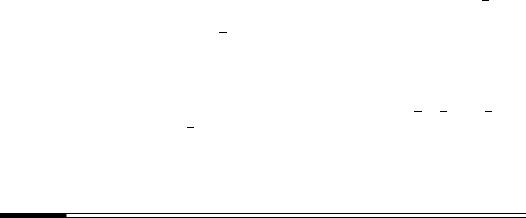
One general technique for destroying the linearity inherent in LFSRs is to use several LFSRs in parallel. The keystream is generated as a nonlinear function Ïof the outputs of the component LFSRs; this construction is illustrated in Figure 6.8. Such keystream generators are called nonlinear combination generators, and Ïis called the combining function. The remainder of this subsection demonstrates that the function Ïmust satisfy several criteria in order to withstand certain particular cryptographic attacks.
LFSR 1 |
|
|
LFSR 2 |
Ï |
keystream |
LFSR n
Figure 6.8: A nonlinear combination generator. lis a nonlinear combining function.
6.48Definition A product of ± distinct variables is called an ±]7porder product of the variables. Every Boolean function ÏÁ7nºn¶» ¶ ¹n+¹U¹ê¶Âcan be written as a modulo ·sum of distinct ±]7porder products of its variables, Ç ç ±\ç©; this expression is called the algebraic normal form of Ï. The nonlinear order of Ïis the maximum of the order of the terms appearing in its algebraic normal form.
For example, the Boolean function ÏÁ7nºn¶»K¶n¼n¶¶n4°¤µ n»² ²n¼ ²n n4² nºn¼n n4has nonlinear order ¬. Note that the maximum possible nonlinear order of a Boolean function in ©variables is ©. Fact 6.49 demonstrates that the output sequence of a nonlinear combination generator has high linear complexity, provided that a combining function Ïof high nonlinear order is employed.
6.49Fact Suppose that ©maximum-length LFSRs, whose lengths 庶延 ¹ å¹U¹ê¶+are pairwise distinct and greater than ·, are combined by a nonlinear function ÏÁ\nº¶n»¶ ¹U¹n+¹f¶(as in Figure 6.8) which is expressed in algebraic normal form. Then the linear complexity of the keystream is ÏÁ¯åº¶å»¶ ¹U¹å+¹ê¶. (The expression ÏÁ¯åº¶å»¶ ¹U¹å+¹ê¶is evaluated over the integers rather than over ý».)
Handbook of Applied Cryptography by A. Menezes, P. van Oorschot and S. Vanstone.
206 |
Ch. 6 Stream Ciphers |
6.50Example (Geffe generator) The Geffe generator, as depicted in Figure 6.9, is defined by three maximum-length LFSRs whose lengths åº, å», å¼are pairwise relatively prime, with nonlinear combining function
Ï º ¶» ¶¼ ° º».²µ"ú» ¼I° º».²» ¼ ²¼K¹
The keystream generatedÁ\nn nhas periodn nÁ·ëÛÁæµÂnûÁ·ë7næµÂnûÁn·ë ænµÂnand linearn complexity
å° åºå»ú å»å¼ú å¼.
LFSR 1
LFSR 2
LFSR 3
qÛ
q |
keystream |
q
Figure 6.9: The Geffe generator.
The Geffe generator is cryptographically weak because information about the states of LFSR 1 and LFSR 3 leaks into the output sequence. To see this, let nºÁ ä¶n»ÂÁ ä¶n¼Âä¶UÐÂÁä  denote the ä]7poutput bits of LFSRs 1, 2, 3 and the keystream, respectively. Then the correlation probability of the sequence nºÁ äto Âthe output sequence ÐÁ äis Â
r |
Ð ° º ° |
r |
» °|µú |
r |
|
r |
¼ ° º |
|
|
|
|
|
» ° Çû |
||||
|
ÁÁä Ân Á ä Â Â |
|
Á7nÁ ä ÂÂ |
|
|
Á\nÁä Â Â |
Á7nÁä Ân Áä ¯ |
|
|
° |
µú µûµ ° |
¸¹ |
|
|
|||
Similarly, rÁÐÁä ° n¼Áä ¯°·¼. For· this· reason,¬ |
despite having high period and mod- |
|||||||
|
|
|
|
|
|
|
|
|
erately high linear complexity, the Geffe generator succumbs to correlation attacks, as de-
6.51Note (correlation attacks) Suppose that © maximum-length LFSRs oº¶o»¶U¹ o¹U¹ê¶+of lengths 庶延U¹ å¹+¹ê¶are employed in a nonlinear combination generator. If the connection polynomials of the LFSRs and the combining function Ïare public knowledge, then
the number of different keys of the generator is  +®^QºÁ·ëÖæµÂ. (A key consists of the initial states of the LFSRs.) Suppose that there is a correlation between the keystream and
the output sequence of oº, with correlation probability sJ@»º. If a sufficiently long segment of the keystream is known (e.g., as is possible under a known-plaintext attack on a binary additive stream cipher), the initial state of oºcan be deduced by counting the number of coincidences between the keystream and all possible shifts of the output sequence of oº, until this number agrees with the correlation probability s. Under these conditions, finding the initial state of oºwill take at most ·ëÛæ µtrials. In the case where there is
a correlation between the keystream and the output sequences of each of oº¶o»¶ ¹U¹o+,¹f¶ the (secret)ë initial state of each LFSR can be determined independently in a total of about
 +®gQºÁ· Öæ µÂtrials; this number is far smaller than the total number of different keys. In a similar manner, correlations between the output sequences of particular subsets of the LFSRs and the keystream can be exploited.
In view of Note 6.51, the combining function Ïshould be carefully selected so that there is no statistical dependence between any small subset of the ©LFSR sequences and
Êc 1997 by CRC Press, Inc. — See accompanying notice at front of chapter.
Ë6.3 Stream ciphers based on LFSRs |
207 |
the keystream. This condition can be satisfied if Ïis chosen to be ±]\p-order correlation immune.
6.52Definition Let t ºt¶» ¶U¹t+¹U¹ê¶be independent binary variables, each taking on the values Çor µwith probability »º. A Boolean function ÏÁ7nº¶n»¶U¹ n¹U¹ê¶+Âis ±]7p-order corre-
lation immune if for each subset of ± random variables t®Û¶t®¶ ¹U¹t®¹ê¶^uwith µ ç´ºG
´» |
û ûUû´Ü ç©, the random variable v °IÏÁ7tº¶t»¶ ¹U¹t+¹f¶Âis statistically indepen- |
G |
G |
dent of the random vector Á7t®Û¶t®¶U¹ t¹®¹3¶\uÂ; equivalently, Å Á?v®.Û¶Ætwt®¶U¹ t¹U¹ê¶®\u°
Ç(see Definition 2.45).
For example, the function ÏÁ7nº¶n»¶U¹ n¹U¹ê¶+° nº² n»² ûUûn+ûis²Á© æµÂ\]\p-
order correlation immune. In light of Fact 6.49, the following shows that there is a tradeoff between achieving high linear complexity and high correlation immunity with a combining function.
6.53 Fact If a Boolean function ÏÁ7nºn¶» ¶U¹n+¹U¹f¶Âis ±]\p-order correlation immune, where µ ç
± ©, then the nonlinear order of Ïis at most © æ±. Moreover, if Ïis balanced (i.e., exactlyG half of the output values of Ïare Ç) then the nonlinear order of Ïis at most ©.±æ æµ
for µ ç7±©wæç·.
The tradeoff between high linear complexity and high correlation immunity can be avoided by permitting memory in the nonlinear combination function Ï. This point is illustrated by the summation generator.
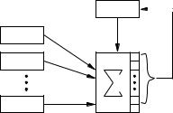
6.54Example (summation generator) The combining function in the summation generator is based on the fact that integer addition, when viewed over ý», is a nonlinear function with
memory áwhoseº correlation immunity is maximum. To see this in the case © ° ,·let x°
xÜáº·Ü ú ûUûxº·KúûxÔand y° yÜặÜáºú ûUûyº·ûúyÔbe the binary representations
of integers xand y. Then the bits of Ðs°xú yare given by the recursive formula:
Ð |
° |
Ϻ |
¶ ¶ Ạ° |
² |
² áº Ç ç ç ± ¶ |
|
é |
° |
Á xyééé Â |
xVéy é é |
ẶÉÇ çç ± µ ¶ |
||
|
Ï» |
¶ ¶ Ạ° |
² |
² |
||
where éiséthe carry Ábit,xandyééé ºá° xxÜVézy° ÁyéÜxVé°yÇé. Note that Ϻis ·æ'{V|-order corre-
lation immune, while Ϧ»is a memoryless nonlinear function. The carry bit éáºcarries all the nonlinear influence of less significant bits of xand y(namely, xéẠ¶ ¹x¹U¹f¶xÔand
yéẠ¶ ¹yº¹U¹f¶y¶Ô).
The summation generator, as depicted in Figure 6.10, is defined by ©maximum-length LFSRs whose lengths åºå¶»K¶ ¹å+¹U¹ê¶are pairwise relatively prime. The secret key con-
LFSR 1
LFSR 2
LFSR n
qÛ q
q~}
Carry
 keystream
Figure 6.10: The summation generator.
Handbook of Applied Cryptography by A. Menezes, P. van Oorschot and S. Vanstone.
208 Ch. 6 Stream Ciphers
sists of the initial states of the LFSRs, and an initial (integer) carry ¾Ô. The keystream is generated as follows. At time ( 7ªµ), the LFSRs are stepped producing output bits nºn¶» ¶ ¹U¹n , and¹ê¶the integer sum é°  ®+^Qºn®ú ¾éáºis computed. The keystream bit is é +·(the least significant bit of é), while the new carry is computed as ¾é° W <é·zA'Y(the remaining bits of <é). The period of the keystream is
  ®+^QºÁ·ëÖæµÂ, while its linear complexity is close to this number.
Even though the summation generator has high period, linear complexity, and correlation immunity, it is vulnerable to certain correlation attacks and a known-plaintext attack based on its ·-adic span (see page 218).
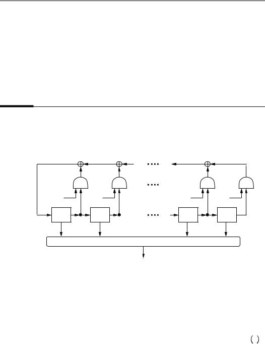
6.3.2 Nonlinear filter generators
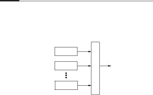
Another general technique for destroying the linearity inherent in LFSRs is to generate the keystream as some nonlinear function of the stages of a single LFSR; this construction is illustrated in Figure 6.11. Such keystream generators are called nonlinear filter generators, and Ïis called the filtering function.
ì¯í îñð |
î ï |
îVòKóQð |
îVò |
Stage |
Stage |
Stage |
Stage |
L-1 |
L-2 |
1 |
0 |
l
keystream
Figure 6.11: A nonlinear filter generator. lis a nonlinear Boolean filtering function.
Fact 6.55 describes the linear complexity of the output sequence of a nonlinear filter generator.
6.55Fact Suppose that a nonlinear filter generator is constructed using a maximum-length LFSR of length åand a filtering function Ïof nonlinear order ± (as in Figure 6.11).
(i)(Key’s bound) The linear complexity of the keystream is at most åÜ ° Ü®gQº ë®.
(ii)For a fixed maximum-length LFSR of prime length å, the fraction of Boolean functions Ïof nonlinear order ± which produce sequences of maximum linear complexity åÜ is
r |
ë |
áºë |
|
ûñ· |
¹ |
whose linear com- |
|
Therefore, for large å, mostÜ 2of the æsågeneratorsÜ9ÁAñÁ¯åproduce ÂJ@sequencesR |
|||
plexity meets the upper bound in (i).
The nonlinear function Ïselected for a filter generator should include many terms of each order up to the nonlinear order of Ï.
Êc 1997 by CRC Press, Inc. — See accompanying notice at front of chapter.

Ë6.3 Stream ciphers based on LFSRs |
209 |
6.56Example (knapsack generator) The knapsack keystream generator is defined by a maxim- um-length LFSR õ1嶾sÁ÷öandÂ÷øa modulus °|·ë. The secret key consists of åknapsack integer weights xºx¶»K¶ ¹U¹xëeach¹ê¶of bitlength å, and the initial state of the LFSR. Re-
call that the subset sum problem (¨3.10) is to determine a subset of the knapsack weights which add up to a given integer è, provided that such a subset exists; this problem is NP- hard (Fact 3.91). The keystream is generated as follows: at time , the LFSR is stepped and the knapsack sum <é°  ®ë^Qºn®x® B is computed, where þnë ¶U¹n»¹nº¹ê¶ÿis the state of the LFSR at time . Finally, selected bits of <é(after <éis converted to its binary representation) are extracted to form part of the keystream (the g leastOå significant bits of <éshould be discarded). The linear complexity of the keystream is then virtually certain
to be åAÁ·ëæ µÂ.
Since the state of an LFSR is a binary vector, the function which maps the LFSR state to the knapsackë sum éis indeed nonlinear. Explicitly, let the function Ïbe defined by
ÏÁ7nR° ®^Qºn®x® _, where% n ° þnë¶ ¹U¹n»K¶¹f¶nºÿis a state. If n and are two
states then, in general, ÏÁ7n² ê°EÁÏ\núRÂÁÏ7. êÂ
6.3.3 Clock-controlled generators
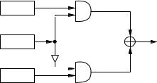
In nonlinear combination generators and nonlinear filter generators, the component LFSRs are clocked regularly; i.e., the movement of data in all the LFSRs is controlled by the same clock. The main idea behind a clock-controlled generator is to introduce nonlinearity into LFSR-based keystream generators by having the output of one LFSR control the clocking (i.e., stepping) of a second LFSR. Since the second LFSR is clocked in an irregular manner, the hope is that attacks based on the regular motion of LFSRs can be foiled. Two clockcontrolled generators are described in this subsection: (i) the alternating step generator and (ii) the shrinking generator.
(i) The alternating step generator
The alternating step generator uses an LFSR oºto control the stepping of two LFSRs, o» and o¼. The keystream produced is the XOR of the output sequences of o»and o¼.
6.57Algorithm Alternating step generator
SUMMARY: a control LFSR oºis used to selectively step two other LFSRs, o»and o¼. OUTPUT: a sequence which is the bitwise XOR of the output sequences of o»and o¼. The following steps are repeated until a keystream of desired length is produced.
1.Register oºis clocked.
2.If the output of oºis µthen:
o»is clocked; o¼is not clocked but its previous output bit is repeated. (For the first clock cycle, the “previous output bit” of o¼is taken to be Ç.)
3. If the output of oºis Çthen:
o¼is clocked; o»is not clocked but its previous output bit is repeated. (For the first clock cycle, the “previous output bit” of o»is taken to be Ç.)
4. The output bits of o»and o¼are XORed; the resulting bit is part of the keystream.
More formally, let the output sequences of LFSRs oº, o», and o¼be xÔx¶ºx¶»K¶,¹ ¹U¹
yÔy¶º¦¶y» ¶,¹U¹and ¹Ô ¶ º, respectively¶ »O¹. Define¹ ¹ yáºN°áº?°|Ç. Then the keystream
produced by the alternating step generator is nÔK¶nºU¶n»K¶,¹U¹where¹né° yâé-²7éá<âéá-º
Handbook of Applied Cryptography by A. Menezes, P. van Oorschot and S. Vanstone.