

Курсовая работа_ф_3 / FreematPrimerV4e1
.pdfWith 32 sections, the total area is 1.977035
The calculated area from -1.000000 to 2.000000 is 1.977035
The total area went up from 1.971305 to 1.977035. Note that the number of steps went up by a factor
of 4. Let's next try an accuracy of precision of 10-6. epsilon=1e-6; % Set the desired accuracy.
Now, let's run the script again.
--> rectAreaPrec
The desired accuracy is 1e-06
With 2 sections, the total area is 1.899024
With 4 sections, the total area is 1.952193
With 8 sections, the total area is 1.971305
With 16 sections, the total area is 1.975899
With 32 sections, the total area is 1.977035
With 64 sections, the total area is 1.977318
With 128 sections, the total area is 1.977389
With 256 sections, the total area is 1.977407
With 512 sections, the total area is 1.977411
With 1024 sections, the total area is 1.977412
The calculated area from -1.000000 to 2.000000 is 1.977412
That took a few more sections. Is there a way to improve the code such that it doesn't take so many computations? Yes. That's where the trapezoid, Simpson's Rule, and the Gaussian quadrature method come into play.
But before we jump into those methods, let's finish this up by making this into a function that we can use for general purposes. The function I'm going to create uses four things as inputs: the equation to be
integrated, the start point, the stop point, and a desired accuracy.
% Function to calculate the area under a curve using the rectangle
% method.
%
% The function will input the following variables:
% - eqn: This will be the equation which will be numerically % integrated.
% It will be entered as an anonymous function.
% - start: This will be the start of the area to be integrated.
% - stop: This will be the end of the area to be integrated.
% - epsilon: This is the desired accuracy for the numerical % integration.
function finalValue=rectz(eqn,start,stop,epsilon)
sects=2;
w=(stop-start)/sects; % calculate the width of the rectangles. x=(start+w/2):w:stop; % calculate the midpoints of each section. area=eqn(x)*w; % calculate the height of each rectangle. totalArea=sum(area); % sum up each section.
lastArea=totalArea; % this variable is used to determine when the % desired accuracy has been reached.
diffErr=totalArea;
while(diffErr>(epsilon*totalArea))
sects=sects*2; % double the number of sections with each iteration. w=(stop-start)/sects;
x=(start+w/2):w:stop;
area=eqn(x)*w;
The Freemat Primer
Page 181 of 218

totalArea=sum(area);
diffErr=abs(lastArea-totalArea); % calculate the difference between the
lastArea=totalArea; end
% consecutive values.
finalValue=totalArea; % read out the final calculated value
I saved this with the filename of rectz.m. Trying this out with a desired accuracy of 10-4, we get:
--> eqn=@(x) (exp(-x.^2)+2.5*exp(-(x-3).^2)); --> rectz(eqn,-1,2,1e-4)
ans = 1.9774
Topic 9.3.1.2 Trapezoid Rule
The idea behind the trapezoid rule is to provide a shape that provides a better "fit" than the rectangular section. The concept is to use trapezoids as opposed to rectangles. In the rectangular method, only one point of each section touches the graph. In the trapezoidal method, both sides of each section touch the graph creating a piecewise linear approximation of the original graph. This is shown in Figure 126.
Figure 126: This is a comparison of the rectangular and trapezoidal methods of numerical integration. Note how the trapezoidal method follows the contour of the graph.
To calculate the area of each section, it's necessary to calculate the area of a trapezoid. This is shown in Figure 127.
The Freemat Primer
Page 182 of 218

Figure 127: Calculation of the area of a trapezoid for numerical integration.
Rather than go through the steps from the previous section, we'll just modify the rectangular method function (saved as rectz.m) for the trapezoidal method. The changes involve the calculation for the area of each section. I've changed the calculation from that of a rectangle to that of a trapezoid. I did use a minor "trick" in the calculation in which I used the circshift function (FD, p. 269) rather than
calculating each section independently. I saved this function as trapz.m. |
|
% Function to calculate the area under a curve using the trapezoid |
|
% method. |
|
% |
|
% The function will input the following variables: |
|
% - eqn: This will be the equation which will be numerically |
|
% |
integrated. |
% It will be entered as an anonymous function. |
|
% - start: This will be the start of the area to be integrated. |
|
% - stop: This will be the end of the area to be integrated. |
|
% - epsilon: This is the desired accuracy for the numerical |
|
% |
integration. |
function finalValue=trapz(eqn,start,stop,epsilon) |
|
sects=2;
w=(stop-start)/sects; % calculate the width of the rectangles. x=start:w:stop; % calculate the edge points of each section. h0=eqn(x); % calculate the height of both edges of each section. h1=circshift(h0,[0,-1]); % rotate the vector to allow adding
The Freemat Primer
Page 183 of 218

% consecutive parts to calculate the area. area=(h0+h1)*w/2; % calculate the area of a trapezoid totalArea=sum(area); % sum up each section. totalArea=areaSum(length(x)-1); % read out the accumulated sum. lastArea=totalArea; % this variable is used to determine when the
diffErr=totalArea;
% desired accuracy has been reached.
while(diffErr>(epsilon*totalArea))
sects=sects*2; % double the number of sections with each iteration. w=(stop-start)/sects;
x=start:w:stop;
h0=eqn(x); h1=circshift(h0,[0,-1]); area=(h0+h1)*w/2; areaSum=cumsum(area); totalArea=areaSum(length(x)-1);
diffErr=abs(lastArea-totalArea); % calculate the difference between the % consecutive values.
lastArea=totalArea; end
finalValue=totalArea; % read out the final calculated value
Testing this new function with the previous equation, we get this:
--> eqn=@(x) (exp(-x.^2)+2.5*exp(-(x-3).^2)); --> trapz(eqn,-1,2,1e-4)
ans =
1.9775
Topic 9.3.1.3 Simpson's Rule
The idea behind Simpson's rule is that rather than using trapezoids to form a piecewise linear approximation of the graph to instead use an equation of the form f x =ax2 bx c . This equation
creates a parabola. Hence, each section will be a piecewise parabolic shape that follows the graph. This is shown in Figure 128.
Figure 128: Comparison of rectangular method and Simpson's rule.
The area for each section is actually a straightforward calculation, as shown in Figure 129. (The
The Freemat Primer
Page 184 of 218

derivation of this calculation is another matter.)
Figure 129: Calculation of the area for each section using Simpson's rule.
Once again, we'll use the original function rectz.m and modify it for the area according to Simpson's rule.
%Function to calculate the area under a curve using Simpsons rule.
%The function will input the following variables:
%- eqn: This will be the equation which will be numerically
%integrated.
%It will be entered as an anonymous function.
%- start: This will be the start of the area to be integrated.
%- stop: This will be the end of the area to be integrated.
%- epsilon: This is the desired accuracy for the numerical
%integration.
function finalValue=quadv(eqn,start,stop,epsilon)
sects=2;
w=(stop-start)/sects; % calculate the width of each section. x=start:w:stop; % calculate the endpoints of each section. xmid=(start+w/2):w:stop; % calculate the midpoint of section. h0=eqn(x); % calculate the height of the beginning of each section. hmid=[eqn(xmid) 0]; % calculate the height of the midpoint of each
% section.
h1=circshift(h0,[0,-1]); % rotate the h0 vector to create another
The Freemat Primer
Page 185 of 218

% vector of the endpoint heights of each
% section.
area=(w/6)*(h0+4*hmid+h1); % calculate the area of each section % according to Simpsons rule.
areaSum=cumsum(area); % sum up each section. totalArea=areaSum(length(x)-1); % read out the accumulated sum. lastArea=totalArea; % this variable is used to determine when the
diffErr=totalArea;
% desired accuracy has been reached.
while(diffErr>(epsilon*totalArea))
sects=sects*2; % double the number of sections with each iteration. w=(stop-start)/sects;
x=start:w:stop; % calculate the endpoints of each section. xmid=(start+w/2):w:stop; % calculate the midpoint of section. h0=eqn(x);
hmid=[eqn(xmid) 0]; h1=circshift(h0,[0,-1]); area=(w/6)*(h0+4*hmid+h1); areaSum=cumsum(area); totalArea=areaSum(length(x)-1);
diffErr=abs(lastArea-totalArea); % calculate the difference between the % consecutive values.
lastArea=totalArea; end
finalValue=totalArea; % read out the final calculated value
Checking this with the previous routines, we get:
--> quadv(eqn,-1,2,1e-4) ans =
1.9774
This is the same as the rectz and trapz routines (used with the rectangular method and the trapezoidal method, respectively).
Topic 9.3.1.4: Gauss-Legendre Method
The concept of the Gaussian quadrature rule is to use "a weighted sum of function values at specified points within the domain of integration."3 In other words, this uses some high-level math to arrive at an answer for a definite integral. In mathematical terms, we're going to use this equation:
b |
n |
|
b−a |
|
a b |
|
|
∫f x dx≈ b−a ∑ wi f |
xi |
||||||
2 |
|
||||||
a |
2 i=1 |
2 |
|||||
What's happening here is that we're calculating the value of our function at several different points, weighting those values, then summing them up. Note that on the right-hand side, the value of xi is determined by the roots of a Legendre polynomial; the values used from the limits of the integral are from the part (a+b)/2, which is the midpoint of each section calculated. Clear as mud?
Rather than calculating the roots of the polynomial, we're going to used already-calculated values for a 5-point polynomial4. These are:
3 From Wikipedia article "Gaussian quadrature", http://en.wikipedia.org/wiki/Gaussian_quadrature, pulled 19 June 2011. 4 From Wikipedia article "Gaussian quadrature", http://en.wikipedia.org/wiki/Gaussian_quadrature, pulled 19 June 2011
The Freemat Primer
Page 186 of 218

n |
|
Root Value |
Weight |
||||||||||||||||||
|
|
|
|
|
|
|
|
|
|
|
|
|
|
|
|
|
|
|
|
|
|
1 |
|
|
|
|
0 |
|
|
|
|
|
|
2 |
|
|
|
|
|
|
|||
|
|
|
|
|
|
|
|
|
|
|
|
|
|
|
|
|
|
|
|
|
|
2 |
|
|
|
|
±1 / |
|
|
|
|
|
|
1 |
|
|
|
|
|
|
|||
|
|
|
|
3 |
|
|
|
|
|
|
|||||||||||
3 |
|
|
|
|
0 |
|
|
|
|
|
|
8/9 |
|
|
|
|
|
|
|||
|
|
|
|
|
|
|
|
|
|
|
|
|
|
|
|
|
|
|
|
|
|
|
|
|
|
|
|
|
|
|
|
|
|
|
5/9 |
|
|
|
|
|
|
||
|
|
|
|
± 3/5 |
|
|
|
|
|
|
|||||||||||
|
|
|
|
|
|
|
|
|
|
|
|||||||||||
4 |
|
|
|
|
|
|
|
|
|
|
|
|
|
18 |
|
|
|
|
|
|
|
|
|
|
|
|
|
|
|
|
|
|
|
|
|
|
|
|
|
|
|||
|
|
|
|
|
|
|
|
|
|
|
|
|
|
|
30 |
|
|
|
|||
|
± |
|
|
3−2 6/5 |
|
|
|||||||||||||||
|
|
|
|
|
|
|
|
|
|
|
|
|
|
|
|
||||||
|
|
|
|
|
7 |
|
|
|
|
|
36 |
|
|
|
|
|
|
||||
|
|
|
|
|
|
|
|
|
|
|
|
|
|
18− |
|
|
|
|
|
|
|
|
|
|
|
|
|
|
|
|
|
|
|
|
|
|
|
|
|
|
|
||
|
|
|
|
|
|
|
|
|
|
|
|
|
|
|
30 |
|
|
|
|||
|
± |
|
|
3 2 6/5 |
|
|
|
|
|
||||||||||||
|
|
|
|
|
|
|
|
|
|
|
|
|
|
||||||||
|
|
|
|
|
7 |
|
|
|
|
|
36 |
|
|
|
|
|
|
||||
|
|
|
|
|
0 |
|
|
|
|
|
|
128/225 |
|
|
|
||||||
|
|
1 |
|
|
|
|
|
|
|
|
|
|
322 13 |
|
|
|
|||||
|
|
|
|
|
|
|
|
|
|
|
|
70 |
|||||||||
|
|
|
|
|
|
|
|
|
|
|
|
||||||||||
|
± |
5−2 10/7 |
|||||||||||||||||||
5 |
3 |
900 |
|
|
|
|
|
|
|||||||||||||
|
|
|
|
|
|
|
|
|
|
|
|
|
|
|
|
|
|
|
|
||
|
|
1 |
|
|
|
|
|
|
|
|
|
|
322−13 |
|
|
||||||
|
|
|
|
|
|
|
|
|
|
|
|
70 |
|||||||||
|
|
|
|
|
|
|
|
|
|
|
|
||||||||||
|
± |
5 2 10/7 |
|||||||||||||||||||
|
3 |
900 |
|
|
|
|
|
|
|||||||||||||
Once again adapting the original code from the rectz.m function, we get this function which we will
name quadgl.m:
% Numerical integration using the Gaussian quadrature method % This routine will use a five-point Gaussian quadrature rule.
function finalValue=quadgl(eqn,a,b,epsilon)
% Setup constants and weights for five-point Gaussian
% quadrature based on Gauss-Legendre polynomial.
c1=(1/3)*(5-2*(10/7)^0.5)^0.5; c2=(1/3)*(5+2*(10/7)^0.5)^0.5; w0=128/225; w1=(322+13*(70)^0.5)/900; w2=(322-13*(70)^0.5)/900;
% Calculate values based on 2 sections.
sects=2; w=(b-a)/sects; wh=w/2; x=(a+wh):w:b;
h=(w0*wh*eqn(x))+(w1*wh*eqn(-wh*c1+x))+(w1*wh*eqn(wh*c1+x))+
(w2*wh*eqn(-wh*c2+x))+(w2*wh*eqn(wh*c2+x)); totalArea=sum(h);
diffErr=totalArea;
lastArea=totalArea;
%Increase the number of sections until the desired
%accuracy is reached.
while (diffErr>(epsilon*totalArea))
The Freemat Primer
Page 187 of 218

sects=sects*2; w=(b-a)/sects; wh=w/2; x=(a+wh):w:b;
h=(w0*wh*eqn(x))+(w1*wh*eqn(-wh*c1+x))+(w1*wh*eqn(wh*c1+x))+
(w2*wh*eqn(-wh*c2+x))+(w2*wh*eqn(wh*c2+x)); totalArea=sum(h); diffErr=abs(totalArea-lastArea); lastArea=totalArea;
end finalValue=totalArea;
Checking this with our double exponential equation and an accuracy of 10-4, we get:
--> eqn=@(x) (exp(-x.^2)+2.5*exp(-(x-3).^2)); --> quadgl(eqn,-1,2,1e-4)
ans =
1.9774
If you're wondering why we are generating so many different routines that provide the same answer, then you're asking a good question. The answer is that we're essentially independently verifying that
we're probably getting a good solution. We tried to integrate the equation e−x2 2.5e− x−3 2
rectangular method, the trapezoidal method, Simpson's rule, and the Gauss-Legendre method. In all cases, we achieved the same solution, approximately 1.9774. That probably means that our routines are working as we hoped. If we had arrived at different answers, then we would probably have wondered about our underlying assumptions.
In practical terms, however, we're going to probably stick with one of these. That will be the one that provides the answer with the fewest possible iterations or sections. The following table provides some examples of the number of iterations of the while loop in order to achieve the desired accuracy. Note that this is not an indication of the total number of calculations required. On a per-iteration basis, the rectangular method uses the fewest calculations, while the Gauss-Legendre requires many. However, by looking at the number of iterations required, we can get an idea of how quickly we converge on an answer. As the table below shows, the Gauss-Legendre method provides the fastest convergence in cases of proper integrals with no discontinuities (the fewest iterations) of the four methods used thus far.
The Freemat Primer
Page 188 of 218
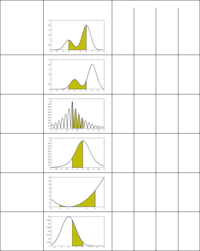
Equation and |
Graph of Equation |
Iterations Required for 10-5 Accuracy |
|||||
|
Limits |
Rect |
Trap |
Simpson |
Gauss |
||
|
|
||||||
|
|
|
|
|
|
|
|
−x2 |
2.5 e |
− x−3 2 |
|
|
|
|
|
e |
|
|
3 |
4 |
3 |
2 |
|
from 0 to 3. |
|
||||||
|
|
|
|
|
|||
−x2 |
− x−3 2 |
|
|
|
|
|
e |
2.5e |
8 |
9 |
4 |
2 |
|
from -1 to 2. |
||||||
|
|
|
|
|||
e− x cos 10x |
10 |
8 |
9 |
8 |
|
from 0 to 1. |
|||||
|
|
|
|
125 |
|
|
|
|
5 2 x−2 2 3 |
7 |
8 |
2 |
2 |
from 1 to 2. |
|
|
|
|
x2 |
9 |
10 |
2 |
2 |
|
from -1 to 3. |
|||||
|
|
|
|
1−x22
|
|
|
e |
7 |
7 |
4 |
2 |
|
|
|
|||||
2 |
from 0.5 to 2.
The Freemat Primer
Page 189 of 218

Topic 9.3.1.5: Monte Carlo Integration
Monte Carlo methods are methods that use random numbers to do different mathematical tasks. Probably the most common usage is for numerical integration, as we'll describe here. This method can work on anything from simple functions to image analysis. Here's how it works:
Say we were to lay out the domain [0 π] onto a dart board, and plot cos(x) on that domain. If we throw a random distribution of darts at this board, it might look like this: (red crosses are darts)
Numerically, the proportion of darts “under the curve” (between the curve and the x-axis) to the total number of darts thrown is equal to the proportion of area under the curve to total area of the domain. Note that darts above the curve but below the x-axis subtract from this total.
Knowing that there are 100 darts in the above figure, we can manually count and come up with 18 darts below the curve in the left half of the graph, and 18 darts above the curve (but below the axis) in the
right half. We subtract this from our first number and get 0. The total area of our domain is 2π, so 0*2π
is the area under the curve. We know, of course, that the value of this integral should be zero, and see that we come up with that here.
Pretty simple, right? Let's look at some simple code then! Let's start by making a function we can pass arguments to. We need to tell it three things: our function (which we can pass as a variable using an anonymous function), the minimum x and the maximum x (the extrema of our domain).
function return_value = montecarlo(fx, xmin, xmax)
n_darts = 100; % number of darts to throw; more darts = more accurate
The Freemat Primer
Page 190 of 218