

Параллельные Процессы и Параллельное Программирование / SNNSv4.2.Manual
.pdf4.3. WINDOWS OF XGUI |
49 |
25.USE : Also opens a menu of loaded pattern sets. The pattern set of the selected entry becomes the current set. All training, testing, and propagation actions refer always to the current pattern set. The name of the corresponding pattern le is displayed next to the button in the Current Pattern Set eld.
26.Current Pattern Set: This eld displays the name of the pattern set currently used for training. When no current pattern set is de ned, the entry "Training Pattern File ?" is displayed.
27.VALID: Gives the intervals in which the training process is to be interrupted by the computation of the error on the validation pattern set. A value of 0 inhibits validation. The validation error is printed on the shell window and plotted in the graph display.
28.USE : Opens the menu of loaded pattern sets. The pattern set of the selected entry becomes the current validation set. The name of the corresponding pattern le is displayed next to the button in the Validation Pattern Set eld.
29.Validation Pattern Set: This eld displays the name of the pattern set currently used for validation. When no current pattern set is de ned the entry "Validation Pattern File ?" is displayed.
30.LEARN: Up to ve elds to specify the parameters of the learning function. The number required and their resp. meaning depend upon the learning function used. Only as many widgets as parameters needed will be displayed, i.e. all widgets visible need to be lled in. A description of the learning functions that are already built in into SNNS is given in section 4.4.
31.SEL. FUNC : in the LEARN row invokes a menu to select a learning function (learning procedure). The following learning functions are currently implemented:
ART1 |
ART1 learning algorithm |
|||||||
ART2 |
ART2 learning algorithm |
|||||||
ARTMAP |
ARTMAP learning algorithm |
|||||||
|
|
|
|
|
|
|
|
(all ART models by Carpenter & Grossberg) |
BBPTT |
Batch-Backpropagation for recurrent networks |
|||||||
BPTT |
Backpropagation for recurrent networks |
|||||||
Backpercolation |
Backpercolation 1 (Mark Jurik) |
|||||||
BackpropBatch |
Backpropagation for batch training |
|||||||
BackpropChunk |
Backpropagation with chunkwise weight update |
|||||||
BackpropMomentum |
Backpropagation with momentum term |
|||||||
BackpropWeightDecay |
Backpropagation with Weight Decay |
|||||||
CC |
Cascade correlation meta algorithm |
|||||||
Counterpropagation |
Counterpropagation (Robert Hecht-Nielsen) |
|||||||
Dynamic |
|
LVQ |
LVQ algorithm with dynamic unit allocation |
|||||
|
||||||||
Hebbian |
Hebbian learning rule |
|||||||
JE |
|
BP |
Backpropagation for Jordan-Elman networks |
|||||
|
||||||||
JE |
|
BP |
|
Momentum |
BackpropMomentum for Jordan-Elman networks |
|||
|
|
|||||||
JE |
|
Quickprop |
Quickprop for Jordan-Elman networks |
|||||
|
||||||||
JE |
|
Rprop |
Rprop for Jordan-Elman networks |
|||||
|
||||||||
|
|
|
|
|
|
|
|
|

50 |
|
|
|
|
|
|
|
|
|
|
|
CHAPTER 4. USING THE GRAPHICAL USER INTERFACE |
|||
|
|
|
|
|
|
|
|
|
|
|
|
|
|
|
|
|
Kohonen |
Kohonen Self Organizing Maps |
|
||||||||||||
|
Monte-Carlo |
Monte-Carlo learning |
|
||||||||||||
|
PruningFeedForward |
Pruning algorithms |
|
||||||||||||
|
QPTT |
Quickprop for recurrent networks |
|
||||||||||||
|
Quickprop |
Quickprop (Scott Fahlman) |
|
||||||||||||
|
RM |
|
delta |
Rumelhart-McClelland's delta rule |
|
||||||||||
|
|
||||||||||||||
|
RadialBasisLearning |
Radial Basis Functions |
|
||||||||||||
|
RBF-DDA |
modi ed Radial Basis Functions |
|
||||||||||||
|
Rprop |
Resilient Propagation learning |
|
||||||||||||
|
SimAnn |
|
SS |
|
error |
Simulated Annealing with SSE computation |
|
||||||||
|
|
|
|||||||||||||
|
SimAnn |
|
WTA |
|
error |
Simulated Annealing with WTA computation |
|
||||||||
|
|
|
|||||||||||||
|
SimAnn |
|
WWTA |
|
error |
Simulated Annealing with WWTA computation |
|
||||||||
|
|
|
|||||||||||||
|
Std |
|
Backpropagation |
\vanilla" Backpropagation |
|
||||||||||
|
|
||||||||||||||
|
TACOMA |
TACOMA meta algorithm |
|
||||||||||||
|
TimeDelayBackprop |
Backpropagation for TDNNs (Alex Waibel) |
|
||||||||||||
|
|
|
|
|
|
|
|
|
|
|
|
|
|
|
|
32.UPDATE: Up to ve elds to specify the parameters of the update function. The number required and their resp. meaning depend upon the update function used. Only as many widgets as parameters needed will be displayed, i.e. all elds visible need to lled in.
33.SEL. FUNC : in the UPDATE row invokes a menu to select an update function. A list of the update functions that are already built in into SNNS and their descriptions is given in section 4.5.
34.INIT: Five elds to specify the parameters of the init function. The number required and their resp. meaning depend upon the init function used. Only as many elds as parameters needed will be displayed, i.e. all elds visible need to be lled in.
35.SEL. FUNC : in the INIT row invokes a menu to select an initialization function. See section 4.6 for a list of the init functions available as well as their description.
36.REMAP: Five elds to specify the parameters of the pattern remapping function. The number required and their resp. meaning depend upon the remapping function used. Only as many elds as parameters needed will be displayed, i.e. all elds visible need to be lled in. In the vast majority of cases you will use the default function "None" that requires no parameters.
37.SEL. FUNC : in the REMAP row invokes a menu to select a pattern remapping function. See section 4.7 for a list of the remapping functions available as well as their description.
4.3.4Info Panel
The info panel displays all data of two units and the link between them. The unit at the beginning of the link is called SOURCE, the other TARGET. One may run sequentially through all connections or sites of the TARGET unit with the arrow buttons and look at the corresponding source units and vice versa.

4.3. WINDOWS OF XGUI |
51 |
Figure 4.13: Info panel
This panel is also very important for editing, since some operations refer to the displayed TARGET unit or (SOURCE!TARGET) link. A default unit can also be created here, whose values (activation, bias, IO-type, subnet number, layer numbers, activation function, and output function) are copied into all selected units of the net.
The source unit of a link can also be speci ed in a 2D display by pressing the middle mouse button, the target unit by releasing it. To select a link between two units the user presses the middle mouse button on the source unit in a 2D display, moves the mouse to the target unit while holding down the mouse button and releases it at the target unit. Now the selected units and their link are displayed in the info panel. If no link exists between two units selected in a 2D display, the TARGET is displayed with its rst link, thereby changing SOURCE.
In table 4.2 the various elds are listed. The elds in the second line of the SOURCE or TARGET unit display the name of the activation function, name of the output function, name of the f-type (if available). The elds in the line LINK have the following meaning: weight, site value, site function, name of the site. Most often only a link weight is available. In this case no information about sites is displayed.
Unit number, unit subnet number, site value, and site function cannot be modi ed. To change attributes of type text, the cursor has to be exactly in the corresponding eld.
There are the following buttons for the units (from left to right):
1.Arrow button  : The button below TARGET selects the rst target unit (of the given source unit) the button below SOURCE selects the rst source unit (of the given target unit)
2.Arrow button  : The button below TARGET selects the next target unit (of the given source unit) the button below SOURCE selects the next source unit (of the given target unit)
3.FREEZE : Unit is frozen, if this button is inverted. Changes become active only after SET is clicked.
4.DEF : The default unit is assigned the displayed values of TARGET and SOURCE (only
52 |
|
CHAPTER 4. |
USING THE GRAPHICAL USER INTERFACE |
|||||
|
|
|
|
|
|
|
|
|
|
Name |
Meaning |
Type |
|
set by |
value range |
|
|
|
|
|
|
|
|
|
|
|
|
no. |
unit no. |
Label |
|
|
|
1..231 |
|
|
subn. |
subnet no. |
Label |
|
|
|
;32736..32735 |
|
|
io |
IO-type |
Label |
|
OPTIONS |
|
I(nput), O(utput), H(idden), |
|
|
|
|
|
|
|
|
D(ual), S(pecial) |
|
|
act. |
activation |
Text |
|
input |
oat |
|
|
|
iact. |
initial act. |
Text |
|
input |
oat |
|
|
|
out. |
output |
Text |
|
input |
oat |
|
|
|
bias |
bias value |
Text |
|
input |
oat |
|
|
|
name |
unit name |
Text |
|
input |
string, starting with letter |
|
|
|
|
|
|
|
|
|
|
|
|
activation function |
Label |
|
OPTIONS |
|
as available |
|
|
|
output function |
Label |
|
|
as available |
|
||
|
|
OPTIONS |
|
|
||||
|
link |
weight |
Text |
|
input |
oat |
|
|
|
site value |
Label |
|
|
|
oat |
|
|
|
site function |
Label |
|
|
|
as available |
|
|
|
site name |
Label |
|
|
|
as available at TARGET |
|
|
|
|
|
|
|
|
|
|
|
Table 4.2: Table of the unit, link and site elds in the Info panel
activation, bias, IO-type, subnet number, layer numbers, activation function and output function).
5. OPTIONS : Calls the following menu:
change io-type |
change the IO-type |
change f-type |
change f-type |
display activation function |
graph of the activation function |
change activation function |
change activation function |
|
note: f-type gets lost! |
display output function |
graph of the output function |
change output function |
change output function |
|
note: f-type gets lost! |
assign layers |
assign unit to layers |
list all sources |
list all predecessors |
list all targets |
list all successors |
6. SET : Only after clicking this button the attributes of the corresponding unit are set to the speci ed value. The unit is also redrawn. Therefore the values can be changed without immediate e ect on the unit.
There exist the following buttons for links (from left to right):
1. : Select rst link of the TARGET unit.
2. : Select next link of the TARGET unit.
3.OPTIONS : Calls the following menu:

4.3. WINDOWS OF XGUI |
53 |
||
|
|
|
|
|
list current site of TARGET |
list of all links of current site. |
|
|
list all sites of TARGET |
list all sites of the TARGET |
|
|
list all links from SOURCE |
list all links starting at SOURCE |
|
|
delete site |
delete displayed site |
|
|
|
note: f-type gets lost! |
|
|
add site |
add new site to TARGET |
|
|
|
note: f-type gets lost! |
|
|
|
|
|
4. SET : Only after clicking this button the link weight is set.
4.3.4.1Unit Function Displays
The characteristic functions of the units can be displayed in a graphic representation. For this purpose separate displays have been created, that can be called by selecting the options display activation function or display output function in the menu under the options button of the target and source unit in the info panel.
Figure 4.14: The logistic activation function in a unit function display
Figure 4.14 shows an example of an activation function. The window header states whether it is an activation or an output function, as well as whether it is the current function of the source or target unit.
The size of the window is as exible as the picture range of the displayed function. The picture range can be changed by using the dialog widgets at the top of the function displays. The size of the window may be changed by using the standard mechanisms of your window manager.
If a new activation or output function has been de ned for the unit, the display window changes automatically to re ect the new situation. Thereby it is easy to get a quick overview of the available functions by opening the function displays and then clicking through the list of available functions (This list can be obtained by selecting select activation function or select output function in the unit menu).

54 |
CHAPTER 4. USING THE GRAPHICAL USER INTERFACE |
4.3.52D Displays
A 2D display or simply display is always part of the user interface. It serves to display the network topology, the units' activations and the weights of the links. Each unit is located on a grid position, which simpli es the positioning of the units. The distance between two grid points (grid width) can be changed from the default 37 pixels to other values in the setup panel.
The current position, i.e. the grid position of the mouse, is also numerically displayed at the bottom of the manager panel. The x-axis is the horizontal line and valid coordinates lie in the range ;32736 . . . +32735 (short integer).
The current version displays units as boxes, where the size of the box is proportional to the value of the displayed attribute. Possible attributes are activation, initial activation, bias, and output. A black box represents a positive value, an empty box a negative value. The size of the unit varies between 16x16 and 0 pixels according to the value of scaleF actor. The parameter scaleFactor has a default value of 1:0, but may be set to values between 0:0 and 2:0 in the setup panel. Each unit can be displayed with two of several attributes. One above the unit and one below the unit. The attributes to be displayed can be selected in the setup panel.
Links are shown as solid lines, with optional numerical display of the weight in the center of the line and/or arrow head pointing to the target unit. These features are optional, because they heavily a ect the drawing speed of the display window.
A display can also be frozen with the button FREEZE (button gets inverted). It is afterwards neither updated anymore2, nor does it accept further editor commands.
An iconi ed display is not updated and therefore consumes (almost) no CPU time. If a window is closed, its dimensions and setup parameters are saved in a stack (LIFO). This means that a newly requested display gets the values of the window assigned that was last closed. For better orientation, the window title contains the subnet number which was speci ed for this display in the setup panel.
4.3.5.1Setup Panel of a 2D Display
Changes to the kind of display of the network can be performed in the Setup panel. All settings become valid only after the button DONE is clicked. The whole display window is then redrawn.
1.Buttons to control the display of unit information: The rst two lines of the Setup panel (units top and units bottom) contain two buttons each to set the unit parameter that can be displayed at the top resp. the bottom of the unit.
The button ON toggles the display of information which can be selected with the button SHOW . The unit name, unit number, or the z-value (3D coordinate) can be displayed above the unit, the activation, initial activation, bias, or output of the
2If a frozen display has to be redrawn, e.g. because an overlapping window was moved, it gets updated. If the network has changed since the freeze, its contents will also have changed!

4.3. WINDOWS OF XGUI |
55 |
Figure 4.15: Setup Panel of a 2D-display.
unit below the unit. The numerical attribute selected with the button SHOW at the bottom of the unit (activation, initial activation, output, or bias) also determines the size of the unit in the graphical representation.
It is usually not advisable to switch o top (number or name), because this information is needed for reference to the info panel. An unnamed unit is always displayed with its number.
2.Buttons to control the display of link information: The third line consists of three buttons to select the display of link data, ON , ;2:35 , ! .
ON determines whether to draw links at all (then ON is inverted),
;2:35 displays link weights at the center of the line representing the link,
! displays arrow heads of the links pointing from source to target unit.
3.LAYERS invokes another popup window to select the display of up to eight di erent layers in the display window. Layers are being stacked like transparent sheets of paper and allow for a selective display of units and links. These layers need NOT correspond with layers of units of the network topology (as in multilayer feed-forward networks), but they may do so. Layers are very useful to display only a selected subset of the network. The display of each layer can be switched on or o independently. A unit may belong to several layers at the same time. The assignment of units to layers can be done with the menu assign layers invoked with the button OPTIONS in the main Info panel.
4.COLOR sets the 2D{display colors. On monochrome terminals, black on white or white on black representation of the network can be selected from a popup menu.

56 |
CHAPTER 4. USING THE GRAPHICAL USER INTERFACE |
On color displays, a color editing window is opened. This window consists of three parts: The palette of available colors at the top, the buttons to select the item to be colored in the lower left region, and the color preview window in the lower right region.
Figure 4.16: Color Setup Panel.
A color is set by clicking rst at the appropriate button ( TEXT , BACKGROUND , or SELECTION ) and then at the desired color in the color palette. The selected setting is immediately displayed in the color preview window. All colors may be set in any order and any number of times. The changes become e ective in the corresponding 2D{display only after both the setup panel and the color edit panel have been dismissed with the DONE button.
5.Sliders for the selection of link display parameters, links positive and links negative:
There are two slidebars to set thresholds for the display of links. When the bubble is moved, the current threshold is displayed in absolute and relative value at the bottom
of the setup panel. Only those links with an absolute value above the threshold are displayed. The range of the absolute values is 0:0 linkT rigger 10:0 (see also paragraph 4.3.5). The trigger values can be set independently for positive and negative weights. With these link thresholds the user can concentrate on the strong connections. Reducing the number of links drawn is an e ective means to speed up the drawing of the displays, since line drawing takes most of the time to display a network.
Note: The links that are not drawn are only invisible. They still remain accessible, i.e. they are a ected by editor operations.
6.units scale: This slidebar sets the parameter scaleFactor for the size of the growing
boxes of the units. Its range is 0:0 scaleF aktor 2:0. A scale factor of 0:5 draws the unit with activation 0:5 with full size. A scale factor of 2:0 draws a unit with activation 1:0 only with half size.
7.grid width: This value sets the width of the grid on which the units are placed. For some nets, changing the default of 37 pixels may be useful, e.g. to be able to
4.3. WINDOWS OF XGUI |
57 |
better position the units in a geometrical pattern. Overlapping tops and bottoms occur if a grid size of less than 35 pixels is selected (26 pixels if units are displayed without numerical values). This overlap, however, does not a ect computation in any way.
8.origin (grid): These two elds determine the origin of the window, i.e. the grid position of the top left corner. There, the left eld represents the x coordinate, the right is the y coordinate. The origin is usually (0, 0). Setting it to (20, 0) moves the display 20 units to the right and 10 units down in the grid.
9.subnet number: This eld adjusts the subnet number to be displayed in this window. Values between ;32736 and +32735 are possible here.
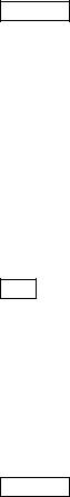
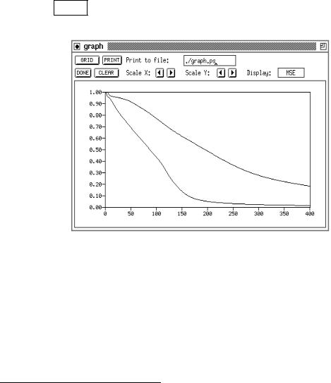
4.3.6Graph Window
Graph is a tool to visualize the error development of a net. The program is started by clicking the graph button in the manager panel or by typing Alt-g in any SNNS window. Figure 4.17 shows the window of the graph tool.
Figure 4.17: Graph window
Graph is only active after calling it. This means, the development of the error is only drawn as long as the window is not closed. The advantage of this implementation is, that the simulator is not slowed down as long as graph is closed3. If the window is iconi ed, graph remains active.
The error curve of the net is plotted until the net is initialized or a new net is loaded, in which case the cycle counter is reset to zero. The window, however, is not cleared until the clear button is pressed. This opens the possibility to compare several error curves in a single display (see also gure 4.17). The maximum number of curves, which can be
3The loss of power by graph should be minimal.

58 |
CHAPTER 4. USING THE GRAPHICAL USER INTERFACE |
displayed simultaneously is 25. If a 26th curve is tried to be drawn, the con rmer appears with an error message.
When the curve reaches the right end of the window, an automatic rescale of the x-axis is performed. This way, the whole curve always remains visible.
In the top region of the graph window, several buttons for handling the display are located:
GRID : toggles the printing of a grid in the display. This helps in comparing di erent curves.
PRINT : Prints the current graph window contents to a Postscript le. If the le already exists a con rmer window pops up to let the user decide whether to overwrite or not. The name of the output le is to be speci ed it the dialog box to the right of the button. If no path is speci ed as pre x, it will be written into the directory xgui was started from.
CLEAR : Clears the screen of the graph window and sets the cycle counter to zero.
DONE : Closes the graph window and resets the cycle counter.
For both the x{ and y{axis the following two buttons are available:
 : Reduce scale in one direction.
  : Enlarge scale in one direction.
SSE : Opens a popup menu to select the value to be plotted. Choices are SSE , MSE ,
and SSE/out , the SSE divided by the number of output units.
While the simulator is working all buttons are blocked.
The graph window can be resized by the mouse like every X-window. Changing the size of the window does not change the size of the scale.
When validation is turned on in the control panel two curves will be drawn simultaneously in the graph window, one for the training set and one for the validation set. On color terminals the validation error will be plotted as solid red line, on B/W terminals as dashed black line.
4.3.7Weight Display
The weight display window is a separate window specialized for displaying the weights of a network. It is called from the manager panel with the WEIGHTS button, or by typing Alt-w in any snns window. On black-and-white screens the weights are represented as squares with changing size in a Hinton diagram, while on color screens, xed size squares with changing colors (WV-diagrams) are used. It can be used to analyze the weight distribution, or to observe the weight development during learning.
Initially the window has a size of 400x400 pixel.The weights are represented by 162 pixels on B/W and 52 pixels on color terminals. If the net is small, the square sizes are automatically enlarged to ll up the window. If the weights do not t into the window, the scrollbars attached to the window allow scrolling over the display.