Параллельные Процессы и Параллельное Программирование / SNNSv4.2.Manual

in German, the most comprehensive and up to date book on neural network learning algorithms, simulation systems and neural hardware is probably [Zel94]

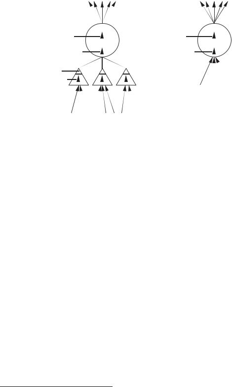
A network consists of units1 and directed, weighted links (connections) between them. In analogy to activation passing in biological neurons, each unit receives a net input that is computed from the weighted outputs of prior units with connections leading to this unit. Picture 3.1 shows a small network.

output unit

6.976.97

input units

Figure 3.1: A small network with three layers of units

The actual information processing within the units is modeled in the SNNS simulator with the activation function and the output function. The activation function rst computes the net input of the unit from the weighted output values of prior units. It then computes the new activation from this net input (and possibly its previous activation). The output function takes this result to generate the output of the unit.2 These functions can be arbitrary C functions linked to the simulator kernel and may be di erent for each unit.

Our simulator uses a discrete clock. Time is not modeled explicitly (i.e. there is no propagation delay or explicit modeling of activation functions varying over time). Rather, the net executes in update steps, where a(t + 1) is the activation of a unit one step after a(t).

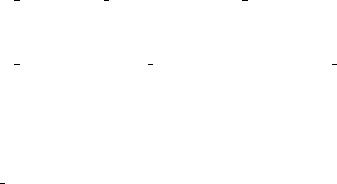
The SNNS simulator, just like the Rochester Connectionist Simulator (RCS, [God87]), o ers the use of sites as additional network element. Sites are a simple model of the dendrites of a neuron which allow a grouping and di erent treatment of the input signals of a cell. Each site can have a di erent site function. This selective treatment of incoming information allows more powerful connectionist models. Figure 3.2 shows one unit with sites and one without.

In the following all the various network elements are described in detail.

3.1.1Units

Depending on their function in the net, one can distinguish three types of units: The units whose activations are the problem input for the net are called input units the units

1In the following the more common name "units" is used instead of "cells".

2The term transfer function often denotes the combination of activation and output function. To make matters worse, sometimes the term activation function is also used to comprise activation and output function.

is inhibitory, i.e. decreasing the activity of the target unit if it is positive, it has an excitatory, i.e. activity enhancing, e ect.

The most frequently used network architecture is built hierarchically bottom-up. The input into a unit comes only from the units of preceding layers. Because of the unidirectionalow of information within the net they are also called feed-forward nets (as example see the neural net classi er introduced in chapter 3.5). In many models a full connectivity between all units of adjoining levels is assumed.

Weights are represented as oats with nine decimal digits of precision.

3.1.3Sites

A unit with sites doesn't have a direct input any more. All incoming links lead to di erent sites, where the arriving weighted output signals of preceding units are processed with di erent user-de nable site functions (see picture 3.2). The result of the site function is represented by the site value. The activation function then takes this value of each site as network input.

The SNNS simulator does not allow multiple connections from a unit to the same input port of a target unit. Connections to di erent sites of the same target units are allowed. Similarly, multiple connections from one unit to di erent input sites of itself are allowed as well.

3.2Update Modes

To compute the new activation values of the units, the SNNS simulator running on a sequential workstation processor has to visit all of them in some sequential order. This order is de ned by the Update Mode. Five update modes for general use are implemented in SNNS. The rst is a synchronous mode, all other are asynchronous, i.e. in these modes units see the new outputs of their predecessors if these have red before them.

1.synchronous: The units change their activation all together after each step. To do this, the kernel rst computes the new activations of all units from their activation functions in some arbitrary order. After all units have their new activation value assigned, the new output of the units is computed. The outside spectator gets the impression that all units have red simultaneously (in sync).

2.random permutation: The units compute their new activation and output function sequentially. The order is de ned randomly, but each unit is selected exactly once in every step.

3.random: The order is de ned by a random number generator. Thus it is not guaranteed that all units are visited exactly once in one update step, i.e. some units may be updated several times, some not at all.

4.serial : The order is de ned by ascending internal unit number. If units are created with ascending unit numbers from input to output units, this is the fastest mode.

Note that the use of serial mode is not advisable if the units of a network are not in ascending order.

5.topological: The kernel sorts the units by their topology. This order corresponds to the natural propagation of activity from input to output. In pure feed-forward nets the input activation reaches the output especially fast with this mode, because many units already have their nal output which doesn't change later.

Additionally, there are 12 more update modes for special network topologies implemented in SNNS.

1.CPN : For learning with counterpropagation.

2.Time Delay: This mode takes into account the special connections of time delay networks. Connections have to be updated in the order in which they become valid in the course of time.

3.ART1 Stable, ART2 Stable and ARTMAP Stable: Three update modes for the three adaptive resonance theory network models. They propagate a pattern through the network until a stable state has been reached.

4.ART1 Synchronous, ART2 Synchronous and ARTMAP Synchronous: Three other update modes for the three adaptive resonance theory network models. They perform just one propagation step with each call.

5.CC : Special update mode for the cascade correlation meta algorithm.

6.BPTT : For recurrent networks, trained with `backpropagation through time'.

7.RM Synchronous: Special update mode for auto-associative memory networks.

Note, that all update modes only apply to the forward propagation phase, the backward phase in learning procedures like backpropagation is not a ected at all.

3.3Learning in Neural Nets

An important focus of neural network research is the question of how to adjust the weights of the links to get the desired system behavior. This modi cation is very often based on the Hebbian rule, which states that a link between two units is strengthened if both units are active at the same time. The Hebbian rule in its general form is:

g(: : :) function, depending on the activation of the unit and the teaching input h(: : :) function, depending on the output of the preceding element and the current

weight of the link

Training a feed-forward neural network with supervised learning consists of the following procedure:

An input pattern is presented to the network. The input is then propagated forward in the net until activation reaches the output layer. This constitutes the so called forward propagation phase.

The output of the output layer is then compared with the teaching input. The error, i.e. the di erence (delta) j between the output oj and the teaching input tj of a target output unit j is then used together with the output oi of the source unit i to compute the necessary changes of the link wij . To compute the deltas of inner units for which no teaching input is available, (units of hidden layers) the deltas of the following layer, which are already computed, are used in a formula given below. In this way the errors (deltas) are propagated backward, so this phase is called backward propagation.

In online learning, the weight changes wij are applied to the network after each training pattern, i.e. after each forward and backward pass. In o ine learning or batch learning the weight changes are cumulated for all patterns in the training le and the sum of all changes is applied after one full cycle (epoch) through the training pattern le.

The most famous learning algorithm which works in the manner described is currently backpropagation. In the backpropagation learning algorithm online training is usually signi cantly faster than batch training, especially in the case of large training sets with many similar training examples.

The backpropagation weight update rule, also called generalized delta-rule reads as follows:

learning factor eta (a constant)

j error (di erence between the real output and the teaching input) of unit j tj teaching input of unit j

oi output of the preceding unit i

i index of a predecessor to the current unit j with link wij from i to j

jindex of the current unit

kindex of a successor to the current unit j with link wjk from j to k

There are several backpropagation algorithms supplied with SNNS: one \vanilla backpropagation" called Std Backpropagation, one with momentum term and at spot elimination called BackpropMomentum and a batch version called BackpropBatch. They can be chosen from the control panel with the button OPTIONS and the menu selection select learning function.

In SNNS, one may either set the number of training cycles in advance or train the network until it has reached a prede ned error on the training set.

3.4Generalization of Neural Networks

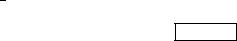
Figure 3.3: Error development of a training and a validation set

One of the major advantages of neural nets is their ability to generalize. This means that a trained net could classify data from the same class as the learning data that it has never seen before. In real world applications developers normally have only a small part of all possible patterns for the generation of a neural net. To reach the best generalization, the dataset should be split into three parts:

The training set is used to train a neural net. The error of this dataset is minimized during training.

The validation set is used to determine the performance of a neural network on patterns that are not trained during learning.

A test set for nally checking the over all performance of a neural net.

Figure 3.3 shows a typical error development of a training set (lower curve) and a validation set (upper curve).

The learning should be stopped in the minimum of the validation set error. At this point the net generalizes best. When learning is not stopped, overtraining occurs and the performance of the net on the whole data decreases, despite the fact that the error on the training data still gets smaller. After nishing the learning phase, the net should benally checked with the third data set, the test set.

SNNS performs one validation cycle every n training cycles. Just like training, validation is controlled from the control panel.

3.5An Example of a simple Network

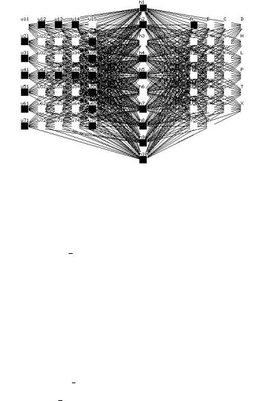
Figure 3.4: Example network of the letter classi er

This paragraph describes a simple example network, a neural network classi er for capital letters in a 5x7 matrix, which is ready for use with the SNNS simulator. Note that this is a toy example which is not suitable for real character recognition.

Network-Files: letters untrained.net, letters.net (trained)

Pattern-File: letters.pat

The network in gure 3.4 is a feed-forward net with three layers of units (two layers of weights) which can recognize capital letters. The input is a 5x7 matrix, where one unit is assigned to each pixel of the matrix. An activation of +1:0 corresponds to \pixel set", while an activation value of 0:0 corresponds to \pixel not set". The output of the network consists of exactly one unit for each capital letter of the alphabet.

The following activation function and output function are used by default:

Activation function: Act logistic

Output function: Out identity

The net has one input layer (5x7 units), one hidden layer (10 units) and one output layer (26 units named 'A' . . . 'Z'). The total of (35 10 + 10 26) = 610 connections form the distributed memory of the classi er.

On presentation of a pattern that resembles the uppercase letter \A", the net produces as output a rating of which letters are probable.