Параллельные Процессы и Параллельное Программирование / SNNSv4.2.Manual

The adaption height and radius are usually decreased over time to enforce the clustering process.

See [Koh88] for a more detailed description of SOMs and their theory.

9.14.2SOM Implementation in SNNS

SNNS originally was not designed to handle units whose location carry semantic information. Therefore some points have to be taken care of when dealing with SOMs. For learning it is necessary to pass the horizontal size of the competitive layer to the learning function, since the internal representation of a map is di erent from its appearance in the display. Furthermore it is not recommended to use the graphical network editor to create or modify any feature maps. The creation of new feature maps should be carried out with the BIGNET (Kohonen) creation tool (see chapter 7).

9.14.2.1The KOHONEN Learning Function

SOM training in SNNS can be performed with the learning function Kohonen. It can be selected from the list of learning functions in the control panel. Five parameters have to be passed to this learning function:

Adaptation Height (Learning Height) The initial adaptation height h(0) can vary between 0 and 1. It determines the overall adaptation strength.

Adaptation Radius (Learning Radius) The initial adaptation radius r(0) is the radius of the neighborhood of the winning unit. All units within this radius are adapted. Values should range between 1 and the size of the map.

Decrease Factor mult H The adaptation height decreases monotonically after the presentation of every learning pattern. This decrease is controlled by the decrease factor mult H: h(t + 1) := h(t) mult H

Decrease Factor mult R The adaptation radius also decreases monotonically after the presentation of every learning pattern. This second decrease is controlled by the decrease factor mult R: r(t + 1) := r(t) mult R

Horizontal size Since the internal representation of a network doesn't allow to determine the 2-dimensional layout of the grid, the horizontal size in units must be provided for the learning function. It is the same value as used for the creation of the network.

Note: After each completed training the parameters adaption height and adaption radius are updated in the control panel to re ect their new values. So when training is started anew, it resumes at the point where it was stopped last. Both mult H and mult R should be in the range (0 1]. A value of 1 consequently keeps the adaption values at a constant level.

9.14.2.2The Kohonen Update Function

A special update function (Kohonen Order) is also provided in SNNS. This function has to be used since it is the only one that takes care of the special ordering of units in the competitive layer. If another update is selected an \Error: Dead units in the network" may occur when propagating patterns.

9.14.2.3The Kohonen Init Function

Before a SOM can be trained, its weights have to be initialized using the init function Kohonen Weights. This init function rst initializes all weights with random values between the speci ed borders. Then it normalizes all links on a per-unit basis. Some of the internal values needed for later training are also set here. It uses the same parameters as CPN Weights (see section 9.6.2).

9.14.2.4The Kohonen Activation Functions

The Kohonen learning algorithm does not use the activation functions of the units. Therefore it is basically unimportant which activation function is used in the SOM. For display and evaluation reasons, however, the two activation functions Act Component and Act Euclid have been implemented in SNNS. Act Euclid copies the Euclidian distance of the unit from the training pattern to the unit activation, while Act Component writes the weight to one speci c component unit into the activation of the unit.

9.14.2.5Building and Training Self-Organizing Maps

Since any modi cation of a Self-Organizing Map in the 2D display like the creation, deletion or movement of units or weights may destroy the relative position of the units in the map we strongly recommend to generate these networks only with the available BIGNET (Kohonen) tool. See also chapter 7 for detailed information on how to create networks. Outside xgui you can also use the tool convert2snns. Information on this program can be found in the respective README le in the directory SNNSv4.2/tools/doc. Note:

Any modi cation of the units after the creation of the network may result in undesired behavior!

To train a new feature map with SNNS, set the appropriate standard functions: select init function KOHONEN Weights, update function Kohonen Order and learning function Kohonen. Remember: There is no special activation function for Kohonen learning, since setting an activation function for the units doesn't a ect the learning procedure. To visualize the results of the training, however, one of the two activation functions Act Euclid and Act Componnent has to be selected. For their semantics see section 9.14.2.6.

After providing patterns (ideally normalized) and assigning reasonable values to the learning function, the learning process can be started. To get a proper appearance of SOMs in the 2D-display set the grid width to 16 and turn o the unit labeling and link display in the display panel.

When a learning run is completed the adaption height and adaption radius parameters are automatically updated in the control panel to re ect the actual values in the kernel.

9.14.2.6Evaluation Tools for SOMs

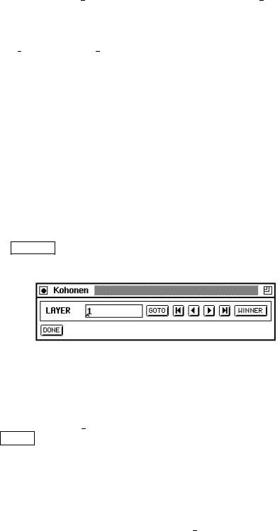
When the results of the learning process are to be analyzed, the tools described here can be used to evaluate the qualitative properties of the SOM. In order to provide this functionality, a special panel was added. It can be called from the manager panel by clicking the KOHONEN button and is displayed in gure 9.13. Yet, the panel can only be used in combination with the control panel.

Figure 9.13: The additional KOHONEN (control) panel

1.Euclidian distance

The distance between an input vector and the weight vectors can be visualized using a distance map. This function allows using the SOM as a classi er for arbitrary input patterns: Choose Act Euclid as activation function for the hidden units, then use the TEST button in the control panel to see the distance maps of consecutive patterns. As green squares (big lled squares on B/W terminals) indicate high activations, green squares here mean big distances, while blue squares represent small distances. Note: The input vector is not normalized before calculating the distance to the competitive units. This doesn't a ect the qualitative appearance of the distance maps, but o ers the advantage of evaluating SOMs that were generated by di erent SOM-algorithms (learning without normalization). If the dot product as similarity measure is to be used select Act Identity as activation function for the hidden units.

the learning layer after the pattern has been propagated a user de ned number of times.

9.15.2Layout of Autoassociative Networks

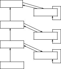
An autoassociative network in SNNS consists of two layers: A layer of world units and a layer of learning units. The representation on the world units indicates the information coming into the network from the outside world. The representation on the learning units represents the network's current interpretation of the incoming information. This interpretation is determined partially by the input and partially by the network's prior learning.

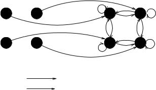
Figure 9.14 shows a simple example network. Each unit in the world layer sends input to exactly one unit in the learning layer. The connected pair of units corresponds to a single node in the typical representation of autoassociative networks. The link from the world unit always has a weight of 1.0, and is unidirectional from the world unit to the learning unit. The learning units are fully interconnected with each other.

Trainable links

Links with fixed weight 1.0

Figure 9.14: A simple Autoassociative Memory Network

The links between the learning units change according to the selected learning rule tot the representation on the world units. The links between the world units and their corresponding learning units are not a ected by learning.

9.15.3Hebbian Learning

In Hebbian learning weights between learning nodes are adjusted so that each weight better represents the relationship between the nodes. Nodes which tend to be positive or negative at the same time will have strong positive weights while those which tend to be opposite will have strong negative weights. Nodes which are uncorrelated will have weights near zero.

The general formula for Hebbian learning is

wij = n inputi inputj

where:

nis the learning rate

inputi is the external input to node i inputj is the external input to node j

9.15.4McClelland & Rumelhart's Delta Rule

This rule is presented in detail in chapter 17 of [RM86]. In general the delta rule outperforms the Hebbian learning rule. The delta rule is also less likely so produce explosive growth in the network. For each learning cycle the pattern is propagated through the network ncycles (a learning parameter) times after which learning occurs. Weights are updated according to the following rule:

wij = n di aj

where:

nis the learning rate

aj is the activation of the source node di is the error in the destination node.

This error is de ned as the external input - the internal input.

In their original work McClelland and Rumelhart used an unusual activation function:

for unit i,

if neti > 0

delta ai = E * neti * (1 - ai) - D * ai else

delta ai = E * neti * (ai + 1) - D * ai

where:

neti is the net input to i (external + internal)

E is the excitation parameter (here set to 0.15)

Dis the decay parameter (here set to 0.15)

This function is included in SNNS as ACT RM. Other activation functions may be used in its place.

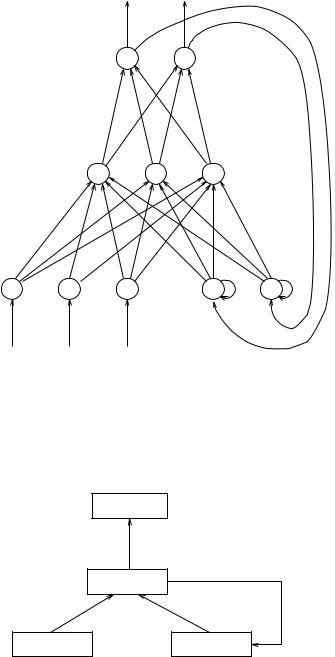
9.16.1.3Extended Hierarchical Elman Networks

Figure 9.17: Extended Elman architecture

9.16.2Working with Partial Recurrent Networks

In this subsection, the initialization, learning, and update functions for partial recurrent networks are described. These functions can not be applied to only the three network models described in the previous subsection. They can be applied to a broader class of partial recurrent networks. Every partial recurrent network, that has the following restrictions, can be used:

If after the deletion of all context units and the links to and from them, the remaining network is a simple feedforward architecture with no cycles.

Input units must not get input from other units.

Outputunits. units may only have outgoing connections to context units, but not to other

Every unit, except the input units, has to have at least one incoming link. For a context unit this restriction is already ful lled when there exists only a self recurrent link. In this case the context unit receives its input only from itself.

In such networks all links leading to context units are considered as recurrent links.

Thereby the user has a lot of possibilities to experiment with a great variety of partial recurrent networks. E.g. it is allowed to connect context units with other context units.

Note: context units are realized as special hidden units. All units of type special hidden are assumed to be context units and are treated like this.

9.16.2.1The Initialization Function JE Weights

The initialization function JE Weights requires the speci cation of ve parameters:

, : The weights of the forward connections are randomly chosen from the interval [ ].

: Weights of self recurrent links from context units to themselves. Simple Elman networks use = 0.

1:0. : Weights of other recurrent links to context units. This value is often set to

: Initial activation of all context units.

These values are to be set in the INIT line of the control panel in the order given above.

9.16.2.2Learning Functions

By deleting all recurrent links in a partial recurrent network, a simple feedforward network remains. The context units have now the function of input units, i.e. the total network input consists of two components. The rst component is the pattern vector, which was the only input to the partial recurrent network. The second component is a state vector. This state vector is given through the next{state function in every step. By this way the behavior of a partial recurrent network can be simulated with a simple feedforward network, that receives the state not implicitly through recurrent links, but as an explicit part of the input vector. In this sense, backpropagation algorithms can easily be modi ed for the training of partial recurrent networks in the following way:

1.Initialization of the context units. In the following steps, all recurrent links are assumed to be not existent, except in step 2(f).

2.Execute for each pattern of the training sequence the following steps:

input of the pattern and forward propagation through the network

calculation of the error signals of output units by comparing the computed output and the teaching output

back propagation of the error signals

calculation of the weight changes

only on{line training: weight adaption

calculation of the new state of the context units according to the incoming links

3.Only o {line training: weight adaption

In this manner, the following learning functions have been adapted for the training of partial recurrent networks like Jordan and Elman networks:

JE BP: Standard Backpropagation for partial recurrent networks