

Параллельные Процессы и Параллельное Программирование / SNNSv4.2.Manual
.pdf9.11. RADIAL BASIS FUNCTIONS (RBFS) |
179 |
function. The scale has been chosen in such a way, that the teaching outputs 0 and 1 are mapped to the input values ;2 and 2.
The optimal values used for 0 scale and 1 scale can not be given in general. With the logistic activation function large scaling values lead to good initialization results, but interfere with the subsequent training, since the logistic function is used mainly in its veryat parts. On the other hand, small scaling values lead to bad initialization results, but produce good preconditions for additional training.
RBF Weights Kohonen One disadvantage of the above initialization procedure is the very simple selection of center vectors from the set of teaching patterns. It would be favorable if the center vectors would homogeneously cover the space of teaching patterns. RBF Weights Kohonen allows a self{organizing training of center vectors. Here, just as the name of the procedure already tells, the self{organizing maps of Kohonen are used (see [Was89]). The simplest version of Kohonen's maps has been implemented. It works as follows:
One precondition for the use of Kohonen maps is that the teaching patterns have to be normalized. This means, that they represent vectors with length 1. K patterns have to be selected from the set of n teaching patterns acting as starting values for the center vectors. Now the scalar product between one teaching pattern and each center vector is computed. If the vectors are normalized to length 1, the scalar product gives a measure for the distance between the two multiplied vectors. Now the center vector is determined whose distance to the current teaching pattern is minimal, i.e. whose scalar product is the largest one. This center vector is moved a little bit in the direction of the current teaching pattern:
~
~znew = ~zold + (l ; ~zold)
This procedure is repeated for all teaching patterns several times. As a result, the center vectors adapt the statistical properties of the set of teaching patterns.
The resp. meanings of the three initialization parameters are:
1.learn cycles: determines the number of iterations of the Kohonen training for all teaching patterns. If 0 epochs are speci ed only the center vectors are set, but no training is performed. A typical value is 50 cycles.
2.learning rate : It should be picked between 0 and 1. A learning rate of 0 leaves the center vectors unchanged. Using a learning rate of 1 replaces the selected center vector by the current teaching pattern. A typical value is 0.4.
3.shu e: Determines the selection of initial center vectors at the beginning of the procedure. A value of 0 leads to the even selection already described for RBF Weights. Any value other than 0 causes a random selection of center vectors from the set of teaching patterns.

180 |
CHAPTER 9. NEURAL NETWORK MODELS AND FUNCTIONS |
Note, that the described initialization procedure initializes only the center vectors (i.e. the link weights between input and hidden layer). The bias values of the neurons have to be set manually using the graphical user interface. To perform the nal initialization of missing link weights, another initialization procedure has been implemented.
RBF Weights Redo This initialization procedure in uences only the link weights between hidden and output layer. It initializes the network as well as possible by taking the bias and the center vectors of the hidden neurons as a starting point. The center vectors can be set by the previously described initialization procedure. Another possibility is to create the center vectors by an external procedure, convert these center vectors into a SNNS pattern le and copy the patterns into the corresponding link weights by using the previously described initialization procedure. When doing this, Kohonen training must not be performed of course.
The e ect of the procedure RBF Weights Redo di ers from RBF Weights only in the way that the center vectors and the bias remain unchanged. As expected, the last two initialization parameters are omitted. The meaning and e ect of the remaining three parameters is identical with the ones described in RBF Weights.
9.11.2.3Learning Functions
Because of the special activation functions used for radial basis functions, a special learning function is needed. It is impossible to train networks which use the activation functions Act RBF : : : with backpropagation. The learning function for radial basis functions implemented here can only be applied if the neurons which use the special activation functions are forming the hidden layer of a three layer feedforward network. Also the neurons of the output layer have to pay attention to their bias for activation.
The name of the special learning function is RadialBasisLearning. The required parameters are:
1.1 (centers): the learning rate used for the modi cation t~j of center vectors according to the formula t~j = ; 1 @@Et~j . A common value is 0:01.
2.2 (bias p): learning rate used for the modi cation of the parameters p of the base
function. p is stored as bias of the hidden units and is trained by the following formula pj = ; 2 @p@Ej . Usualy set to 0:0
3.3 (weights): learning rate which in uences the training of all link weights that are leading to the output layer as well as the bias of all output neurons. A common value is 0:01.
|
@E |
|
@E |
@E |
cj k = ; 3 |
|
di k = ; 3 |
|
bk = ; 3 @bk |
@cj k |
@di k |
4.delta max.: To prevent an overtraining of the network the maximally tolerated error in an output unit can be de ned. If the actual error is smaller than delta max. the corresponding weights are not changed. Common values range from 0 to 0:3.

9.11. RADIAL BASIS FUNCTIONS (RBFS) |
181 |
5.momentum: momentum term during training, after the formula gt+1 = ; 5 @E@g +gt. The momentum{term is usually chosen between 0:8 and 0:9.
The learning rates 1 to 3 have to be selected very carefully. If the values are chosen too large (like the size of values for backpropagation) the modi cation of weights will be too extensive and the learning function will become unstable. Tests showed, that the learning procedure becomes more stable if only one of the three learning rates is set to a value bigger than 0. Most critical is the parameter bias (p), because the base functions are fundamentally changed by this parameter.
Tests also showed that the learning function working in batch mode is much more stable than in online mode. Batch mode means that all changes become active not before all learning patterns have been presented once. This is also the training mode which is recommended in the literature about radial basis functions. The opposite of batch mode is known as online mode, where the weights are changed after the presentation of every single teaching pattern. Which mode is to be used can be de ned during compilation of SNNS. The online mode is activated by de ning the C macro RBF INCR LEARNING during compilation of the simulator kernel, while batch mode is the default.
9.11.3Building a Radial Basis Function Application
As a rst step, a three{layer feedforward network must be constructed with full connectivity between input and hidden layer and between hidden and output layer. Either the graphical editor or the tool BIGNET (both built into SNNS) can be used for this purpose.
The output function of all neurons is set to Out Identity. The activation function of all hidden layer neurons is set to one of the three special activation functions Act RBF : : :
(preferably to Act RBF Gaussian). For the activation of the output units, a function is needed which takes the bias into consideration. These functions are Act Logistic and
Act IdentityPlusBias.
The next step consists of the creation of teaching patterns. They can be generated manually using the graphical editor, or automatically from external data sets by using an appropriate conversion program. If the initialization procedure RBF Weights Kohonen is going to be used, the center vectors should be normalized to length 1, or to equal length.
It is necessary to select an appropriate bias for the hidden units before the initialization is continued. Therefore, the link weights between input and hidden layer are set rst, using the procedure RBF Weights Kohonen so that the center vectors which are represented by the link weights form a subset of the available teaching patterns. The necessary initialization parameters are: learn cycles = 0, learning rate = 0:0, shu e = 0:0. Thereby teaching patterns are used as center vectors without modi cation.
To set the bias, the activation of the hidden units is checked for di erent teaching patterns by using the button TEST of the SNNS control panel. When doing this, the bias of the hidden neurons have to be adjusted so that the activations of the hidden units are as diverse as possible. Using the Gaussian function as base function, all hidden units are uniformly highly activated, if the bias is chosen too small (the case bias = 0 leads to an activation of 1 of all hidden neurons). If the bias is chosen too large, only the unit is activated whose
182 |
CHAPTER 9. NEURAL NETWORK MODELS AND FUNCTIONS |
link weights correspond to the current teaching pattern. A useful procedure to nd the right bias is to rst set the bias to 1, and then to change it uniformly depending on the behavior of the network. One must take care, however, that the bias does not become negative, since some implemented base functions require the bias to be positive. The optimal choice of the bias depends on the dimension of the input layer and the similarity among the teaching patterns.
After a suitable bias for the hidden units has been determined, the initialization procedure RBF Weights can be started. Depending on the selected activation function for the output layer, the two scale parameters have to be set (see page 178). When Act IdentityPlusBias is used, the two values 0 and 1 should be chosen. For the logistic activation function Act Logistic the values -4 and 4 are recommended (also see gure 9.6). The parameters smoothness and deviation should be set to 0 rst. The bias is set to the previously determined value. Depending on the number of teaching patterns and the number of hidden neurons, the initialization procedure may take rather long to execute. Therefore, some processing comments are printed on the terminal during initialization.
After the initialization has nished, the result may be checked by using the TEST button. However, the exact network error can only be determined by the teaching function. Therefore, the learning function RadialBasisLearning has to be selected rst. All learning parameters are set to 0 and the number of learning cycles (CYCLES) is set to 1. After
pressing the button ALL , the learning function is started. Since the learning parameters are set to 0, no changes inside the network will occur. After the presentation of all available teaching patterns, the actual error is printed to the terminal. As usual, the error is de ned as the sum of squared errors of all output units (see formula 9.4). Under certain conditions it can be possible that the error becomes very large. This is mostly due to numerical problems. A poorly selected bias, for example, has shown to be a di cult starting point for the initialization. Also, if the number of teaching patterns is less than or equal to the number of hidden units a problem arises. In this case the number of unknown weights plus unknown bias values of output units exceeds the number of teaching patterns, i.e. there are more unknown parameters to be calculated than equations available. One or more neurons less inside the hidden layer then reduces the error considerably.
After the rst initialization it is recommended to save the current network to test the possibilities of the learning function. It has turned out that the learning function becomes quickly unstable if too large learning rates are used. It is recommended to rst set only one of the three learning rates (centers, bias (p), weights) to a value larger than 0 and to check the sensitivity of the learning function on this single learning rate. The use of the parameter bias (p) is exceptionally critical because it causes serious changes of the base function. If the bias of any hidden neuron is getting negative during learning, an appropriate message is printed to the terminal. In that case, a continuing meaningful training is impossible and the network should be reinitialized.
Immediately after initialization it is often useful to train only the link weights between hidden and output layer. Thereby the numerical inaccuracies which appeared during initialization are corrected. However, an optimized total result can only be achieved if also the center vectors are trained, since they might have been selected disadvantageously.
The initialization procedure used for direct link weight calculation is unable to calculate the

9.12. DYNAMIC DECAY ADJUSTMENT FOR RBFS (RBF{DDA) |
183 |
weights between input and output layer. If such links are present, the following procedure is recommended: Even before setting the center vectors by using RBF Weights Kohonen, and before searching an appropriate bias, all weights should be set to random values between ;0:1 and 0:1 by using the initialization procedure Randomize Weights. Thereby, all links between input and output layer are preinitialized. Later on, after executing the procedure RBF Weights, the error of the network will still be relatively large, because the above mentioned links have not been considered. Now it is easy to train these weights by only using the teaching parameter weights during learning.
9.12Dynamic Decay Adjustment for RBFs (RBF{DDA)
9.12.1The Dynamic Decay Adjustment Algorithm
The Dynamic Decay Adjustment (DDA{)Algorithm is an extension of the RCE-Algorithm (see [Hud92, RCE82]) and o ers easy and constructive training for Radial Basis Function Networks. RBFs trained with the DDA-Algorithm often achieve classi cation accuracy comparable to Multi Layer Perceptrons (MLPs)5 but training is signi cantly faster ([BD95]).
An RBF trained with the DDA-Algorithm (RBF-DDA) is similar in structure to the common feedforward MLP with one hidden layer and without shortcut connections:
The number of units in the input layer represents the dimensionality of the input space.
The hidden layer contains the RBF units. Units are added in this layer during training. The input layer is fully connected to the hidden layer.
Each unit in the output layer represents one possible class, resulting in an 1-of-n or binary coding. For classi cation a winner-takes-all approach is used, i.e. the output with the highest activation determines the class. Each hidden unit is connected to exactly one output unit.
The main di erences to an MLP are the activation function and propagation rule of the hidden layer: Instead of using a sigmoid or another nonlinear squashing function, RBFs use localized functions, radial Gaussians, as an activation function. In addition, a computation of the Euclidian distance to an individual reference vector replaces the scalar product used in MLPs:
Ri(~x) = exp(;jjx~ ;2~rijj2 )i
If the network receives vector ~x as an input, Ri indicates the activation of one RBF unit with reference vector ~ri and standard deviation i.
5As usual the term MLP refers to a multilayer feedforward network using the scalar product as a propagation rule and sigmoids as transfer functions.
184 |
CHAPTER 9. NEURAL NETWORK MODELS AND FUNCTIONS |
The output layer computes the output for each class as follows:
m
f(~x) = XAi Ri(~x)
i=1
with m indicating the number of RBFs belonging to the corresponding class and Ai being the weight for each RBF.
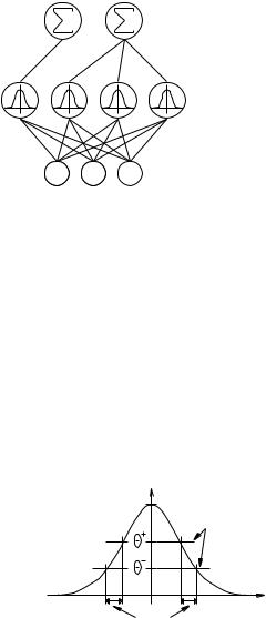
An example of a full RBF-DDA is shown in gure 9.7. Note that there do not exist any shortcut connections between input and output units in an RBF-DDA.
output units
weighted connections
RBF units
input nodes
Figure 9.7: The structure of a Radial Basis Function Network.
In this illustration the weight vector that connects all input units to one hidden unit represents the centre of the Gaussian. The Euclidian distance of the input vector to this reference vector (or prototype) is used as an input to the Gaussian which leads to a local response if the input vector is close to the prototype, the unit will have a high activation. In contrast the activation will be close to zero for larger distances. Each output unit simply computes a weighted sum of all activations of the RBF units belonging to the corresponding class.
The DDA-Algorithm introduces the idea of distinguishing between matching and con icting neighbors in an area of con ict. Two thresholds + and ; are introduced as illustrated in gure 9.8.
 R(x)
R(x)
1.0
thresholds
x
area of conflict
Figure 9.8: One RBF unit as used by the DDA-Algorithm. Two thresholds are used to de ne an area of con ict where no other prototype of a con icting class is allowed to exist. In addition, each training pattern has to be in the inner circle of at least one prototype of the correct class.

9.12. DYNAMIC DECAY ADJUSTMENT FOR RBFS (RBF{DDA) |
185 |
Normally, + is set to be greater than ; which leads to a area of con ict where neither matching nor con icting training patterns are allowed to lie6. Using these thresholds, the algorithm constructs the network dynamically and adjusts the radii individually.
In short the main properties of the DDA-Algorithm are:
constructive training: new RBF nodes are added whenever necessary. The network is built from scratch, the number of required hidden units is determined during training. Individual radii are adjusted dynamically during training.
fast training: usually about ve epochs are needed to complete training, due to the constructive nature of the algorithm. End of training is clearly indicated.
guaranteed convergence: the algorithm can be proven to terminate.
two uncritical parameters: only the two parameters + and ; have to be adjusted manually. Fortunately the values of these two thresholds are not critical to determine. For all tasks that have been used so far, + = 0:4 and ; = 0:2 was a good choice.
guaranteed properties of the network: it can be shown that after training has terminated, the network holds several conditions for all training patterns: wrong classi cations are below a certain threshold ( ;) and correct classi cations are above another threshold ( + ).
The DDA-Algorithm is based on two steps. During training, whenever a pattern is misclassi ed, either a new RBF unit with an initial weight = 1 is introduced (called commit) or the weight of an existing RBF (which covers the new pattern) is incremented. In both cases the radii of con icting RBFs (RBFs belonging to the wrong class) are reduced (called shrink). This guarantees that each of the patterns in the training data is covered by an RBF of the correct class and none of the RBFs of a con icting class has an inappropriate response.
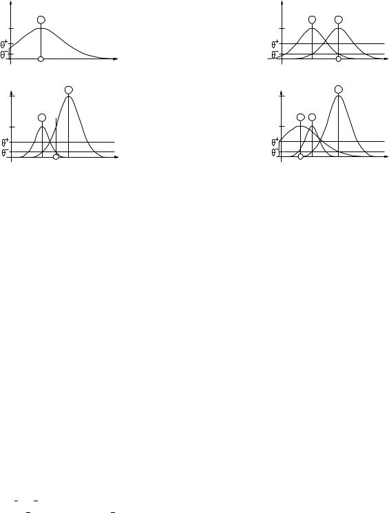
Two parameters are introduced at this stage, a positive threshold + and a negative threshold ;. To commit a new prototype, none of the existing RBFs of the correct class has an activation above + and during shrinking no RBF of a con icting class is allowed to have an activation above ;. Figure 9.9 shows an example that illustrates the rst few training steps of the DDA-Algorithm.
After training is nished, two conditions are true for all input{output pairs7 (~x c) of the training data:
at least one prototype of the correct class c has an activation value greater or equal to +:
9i : Ric(~x) +
all prototypes of con icting classes have activations less or equal to ; (mk indicates
6The only exception to this rule is the case where a pattern of the same class lies in the area of con ict but is covered by another RBF (of the correct class) with a su ciently high activation.
7In this case the term \input{class pair" would be more justi ed, since the DDA{Algorithm trains the network to classify rather than approximate an input{output mapping.
186 |
CHAPTER 9. NEURAL NETWORK MODELS AND FUNCTIONS |
 p(x)
p(x)
A
+1
pattern class A |
x |
|
|
||
|
|
(1) |
+2 p(x) |
B |
|
|
|
|
A |
|
+1 |
|
pattern class B |
x |
|
(3)
 p(x)
p(x)
A |
B |
|
+1 |
|
|
pattern class B |
x |
|
(2)
+2 p(x) |
B |
|
|
|
|
A A |
|
|
+1 |
|
|
pattern class A |
x |
|
|
||
(4)
Figure 9.9: An example of the DDA-Algorithm: (1) a pattern of class A is encountered and a new RBF is created (2) a training pattern of class B leads to a new prototype for class B and shrinks the radius of the existing RBF of class A (3) another pattern of class B is classi ed correctly and shrinks again the prototype of class A (4) a new pattern of class A introduces another prototype of that class.
the number of prototypes belonging to class k):
8k 6= c 1 j mk : Rkj (~x) ;
For all experiments conducted so far, the choice of +=0.4 and ;=0.2 led to satisfactory results. In theory, those parameters should be dependent on the dimensionality of the feature space but in practice the values of the two thresholds seem to be uncritical. Much more important is that the input data is normalized. Due to the radial nature of RBFs each attribute should be distributed over an equivalent range. Usually normalization into [0,1] is su cient.
9.12.2Using RBF{DDA in SNNS
The implementation of the DDA-Algorithm always uses the Gaussian activation function Act RBF Gaussian in the hidden layer. All other activation and output functions are set to Act Identity and Out Identity, respectively.
The Learning function has to be set to RBF-DDA. No Initialization or Update functions are needed.
The algorithm takes three arguments that are set in the rst three elds of the LEARN row in the control panel. These are +, ; (0 < ; + < 1) and the maximum number of RBF
9.13. ART MODELS IN SNNS |
187 |
units to be diplayed in one row. This last item allows the user to control the appearance of the network on the screen and has no in uence on the performance. Specifying 0.0 leads to the default values + = 0:4, ; = 0:2 and to a maximum number of 20 RBF units displayed in a row.
Training of an RBF starts with either:
an empty network, i.e. a network consisting only of input and output units. No connections between input and output units are required, hidden units will be added during training. This can easily be generated with the tool BIGNET (choice FEED FORWARD)
a pretrained network already containing RBF units generated in an earlier run of RBF-DDA (all networks not complying with the speci cation of an RBF-DDA will be rejected).
After having loaded a training pattern set, a learning-epoch can be started by pressing the ALL button in the control panel. At the beginning of each epoch, the weights between the hidden and the output layer are automatically set to zero. Note that the resulting RBF and the number of required learning epochs can vary slightly depending on the order of the training patterns. If you train using a single pattern (by pressing the SINGLE button) keep in mind that every training step increments the weight between the RBF unit of the correct class covering that pattern and its corresponding output unit. The end of the training is reached when the network structure does not change any more and the Mean Square Error (MSE) stays constant from one epoch to another.
The rst desired value in an output pattern that is greater than 0.0 will be assumed to represent the class this pattern belongs to only one output may be greater than 0.0. If there is no such output, training is still executed, but no new prototype for this pattern is commited. All existing prototypes are shrunk to avoid coverage of this pattern, however. This can be an easy way to de ne an \error"{class without trying to model the class itself.
9.13ART Models in SNNS
This section will describe the use of the three ART models ART1, ART2 and ARTMAP, as they are implemented in SNNS. It will not give detailed information on the Adaptive Resonance Theory. You should already know the theory to be able to understand this chapter. For the theory the following literature is recommended:
[CG87a] Original paper, describing ART1 theory. [CG87b] Original paper, describing ART2 theory. [CG91] Original paper, describing ARTMAP theory.
[Her92] Description of theory, implementation and application of the ART models in SNNS (in German).
There will be one subsection for each of the three models and one subsection describing the required topologies of the networks when using the ART learning-, updateor initialization-functions. These topologies are rather complex. For this reason the network
188 |
CHAPTER 9. NEURAL NETWORK MODELS AND FUNCTIONS |
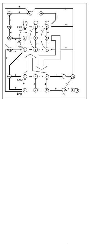
Figure 9.10:
Structure of an ART1 network in SNNS. Thin arrows represent a connection from one unit to another. Fat arrows which go from a layer to a unit indicate that each unit of the layer is connected to the target unit. Similarly a fat arrow from a unit to a layer means that the source unit is connected to each of the units in the target layer. The two big arrows in the middle represent the full connection between comparison and recognition layer and the one between delay and comparison layer, respectively.
creation tool BigNet has been extended. It now o ers an easy way to create ART1, ART2 and ARTMAP networks according to your requirements. For a detailed explanation of the respective features of BigNet see chapter 7.
9.13.1ART1
9.13.1.1Structure of an ART1 Network
The topology of ART1 networks in SNNS has been chosen to to perform most of the ART1 algorithm within the network itself. This means that the mathematics is realized in the activation and output functions of the units. The idea was to keep the propagation and training algorithm as simple as possible and to avoid procedural control components.
In gure 9.10 the units and links of ART1 networks in SNNS are displayed.
The F0 or input layer (labeled inp in gure 9.10) is a set of N input units. Each of them has a corresponding unit in the F1 or comparison layer (labeled cmp). The M elements in the F2 layer are split into three levels. So each F2 element consists of three units. One recognition (rec) unit, one delay (del) unit and one local reset (rst) unit. These three parts are necessary for di erent reasons. The recognition units are known from the theory. The delay units are needed to synchronize the network correctly8 . Besides, the activated unit in the delay layer shows the winner of F2. The job of the local reset units is to block the actual winner of the recognition layer in case of a reset.
8This is only important for the chosen realization of the ART1 learning algorithm in SNNS