

Параллельные Процессы и Параллельное Программирование / SNNSv4.2.Manual
.pdf9.9. THE CASCADE CORRELATION ALGORITHMS |
159 |
An example illustrating this relation is given with the delayed XOR network in the network le xor-rec.net and the pattern les xor-rec1.pat and xor-rec2.pat. With the patterns xor-rec1.pat, the task is to compute the XOR function of the previous input pattern. In xor-rec2.pat, there is a delay of 2 patterns for the result of the XOR of the input pattern. Using a xed network topology with shortcut connections, the BPTT learning algorithm develops solutions with a di erent number of processing steps using the shortcut connections from the rst hidden layer to the output layer to solve the task in xor-rec1.pat. To map the patterns in xor-rec2.pat the result is rst calculated in
the second hidden layer and copied from there to the output layer during the next update step3.
The update function BPTT-Order performs the synchronous update of the network and detects reset patterns. If a network is tested using the TEST button in the control panel, the internal activations and the output activation of the output units are rst overwritten with the values in the target pattern, depending on the setting of the button SHOW . To provide correct activations on feedback connections leading out of the output units in the following network update, all output activations are copied to the units initial activation values i act after each network update and are copied back from i act to out before each update. The non-input activation values may therefore be in uenced before a network update by changing the initial activation values i act.
If the network has to be reset by stepping over a reset pattern with the TEST button,
keep in mind that after clicking TEST , the pattern number is increased rst, the new input pattern is copied into the input layer second, and then the update function is called. So to reset the network, the current pattern must be set to the pattern directly preceding the reset pattern.
9.9The Cascade Correlation Algorithms
Two cascade correlation algorithms have been implemented in SNNS, Cascade-Correlation and recurrent Cascade-Correlation. Both learning algorithms have been developed by Scott Fahlman ([FL91], [HF91], [Fah91]). Strictly speaking the cascade architecture represents a kind of meta algorithm, in which usual learning algorithms like Backprop, Quickprop or Rprop are embedded. Cascade-Correlation is characterized as a constructive learning rule. It starts with a minimal network, consisting only of an input and an output layer. Minimizing the overall error of a net, it adds step by step new hidden units to the hidden layer.
Cascade-Correlation is a supervised learning architecture which builds a near minimal multi-layer network topology. The two advantages of this architecture are that there is no need for a user to worry about the topology of the network, and that Cascade-Correlation learns much faster than the usual learning algorithms.
3If only an upper bound n for the number of processing steps is known, the input patterns may consist of windows containing the current input pattern together with a sequence of the previous n ; 1 input patterns. The network then develops a focus to the sequence element in the input window corresponding to the best number of processing steps.
160 |
CHAPTER 9. NEURAL NETWORK MODELS AND FUNCTIONS |
9.9.1Cascade-Correlation (CC)
9.9.1.1The Algorithm
Cascade-Correlation (CC) combines two ideas: The rst is the cascade architecture, in which hidden units are added only one at a time and do not change after they have been added. The second is the learning algorithm, which creates and installs the new hidden units. For each new hidden unit, the algorithm tries to maximize the magnitude of the correlation between the new unit's output and the residual error signal of the net.
The algorithm is realized in the following way:
1.CC starts with a minimal network consisting only of an input and an output layer. Both layers are fully connected.
2.Train all the connections ending at an output unit with a usual learning algorithm until the error of the net no longer decreases.
3.Generate the so-called candidate units. Every candidate unit is connected with all input units and with all existing hidden units. Between the pool of candidate units and the output units there are no weights.
4.Try to maximize the correlation between the activation of the candidate units and the residual error of the net by training all the links leading to a candidate unit. Learning takes place with an ordinary learning algorithm. The training is stopped when the correlation scores no longer improves.
5.Choose the candidate unit with the maximum correlation, freeze its incoming weights and add it to the net. To change the candidate unit into a hidden unit, generate links between the selected unit and all the output units. Since the weights leading to the new hidden unit are frozen, a new permanent feature detector is obtained. Loop back to step 2.
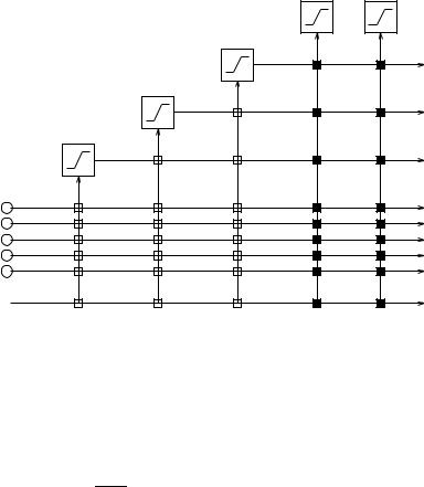
This algorithm is repeated until the overall error of the net falls below a given value. Figure 9.2 shows a net after 3 hidden units have been added.
9.9.1.2Mathematical Background
The training of the output units tries to minimize the sum-squared error E:
E = |
X |
1 |
X |
(ypo ; tpo)2 |
2 |
||||
|
p |
|
o |
|
where tpo is the desired and ypo is the observed output of the output unit o for a pattern p. The error E is minimized by gradient decent using
9.9. THE CASCADE CORRELATION ALGORITHMS |
161 |
|
Outputs |
Output Units |
|
Hidden Unit 3
|
Hidden Unit 2 |
|
Hidden Unit 1 |
Inputs |
|
Bias |
1 |
|
Figure 9.2: A neural net trained with cascade-correlation after 3 hidden units have been added. The vertical lines add all incoming activations. Connections with white boxes are frozen. The black connections are trained repeatedly.
epo = (ypo ; tpo)fp0 (neto)
@E
@wio = Xp epoIip
where fp0 is the derivative of an activation function of a output unit o and Iip is the value of an input unit or a hidden unit i for a pattern p. wio denominates the connection between an input or hidden unit i and an output unit o.
After the training phase the candidate units are adapted, so that the correlation C between the value ypo of a candidate unit and the residual error epo of an output unit becomes maximal. The correlation is given by Fahlman with:
C = |
X X |
(ypo ; yo)(epo ; eo) |
|
|||||
|
o |
p |
|
X |
|
|
|
|
= |
X X |
ypoepo ; eo |
ypo |
|
||||
|
o |
p |
|
p |
|
|
|
|
|
X X |
|
|
|
|
|
|
|
= |
o |
p |
ypo(epo ; eo) |
|
|
|
|
|
|
|
|
|
|
|
|
||
where yo is the average activation of a candidate unit and eo is the average error of an output unit over all patterns p. The maximization of C proceeds by gradient ascent using

162 |
CHAPTER 9. NEURAL NETWORK MODELS AND FUNCTIONS |
p = |
X |
o (epo |
; |
ej)f0 |
|
|
|
|
|
|
p |
|
|
o |
|
|
|
@C |
= |
X |
pIpi |
|
|
@wi |
|
|
|||
|
p |
|
|
|
|
|
|
|
|
|
|
where o is the sign of the correlation between the candidate unit's output and the residual error at output o.
9.9.2Modi cations of Cascade-Correlation
One problem of Cascade-Correlation is the topology of the result net. Since every hidden unit has a connection to every other hidden unit, it's di cult to parallelize the net. The following modi cations of the original algorithm could be used to reduce the number of layers in the resulting network.
The additional parameters needed by the modi cations can be entered in the additional parameter elds in the cascade window. For informations about these values see table 9.2 and the following chapters.
|
modi cation |
no |
param. |
description |
|
|
|
|
|
|
|
|
|
|
SDCC |
1 |
0:0 |
multiplier correlation of sibbling units |
|
|
|
|
|
|
|
||
|
LFCC |
1 |
1 < k |
maximum Fan-In |
|
|
|
|
1 |
|
b |
width of the rst hidden layer |
|
|
|
|
|
|
|
|
|
static |
2 |
|
b |
maximum random di erence to calculated width |
|
|
|
|
|
|
|
|
|
|
3 |
|
d |
exponential growth |
|
|
|
|
|
|
|
|
|
ECC |
1 |
0:0 m 1:0 |
exponential growth |
|
|
|
|
|
|
|
||
|
RLCC |
1 |
0:0 f |
multiplier (powered with neg. layer depth) |
|
|
|
|
|
|
|
||
|
GCC |
1 |
2 g |
no nc |
no of groups |
|
|
|
|
|
|
||
|
|
1 |
0 |
N |
no of runs of the kohonen-map |
|
|
|
|
|
|
|
|
|
|
2 |
0:0 |
step width training of window function |
|
|
|
|
|
|
|
||
|
TACOMA |
3 |
< 1:0 |
if error in region is bigger than , install unit |
|
|
|
|
|
|
|
|
|
|
|
4 |
0:0 1:0 |
if correlation of windows is bigger then |
|
|
|
|
|
|
|
then connect units |
|
|
|
5 |
0:0 < < 1:0 |
initial radius of windows |
|
|
|
|
|
|
|
|
|
Table 9.2: Table of the additional parameters needed by the modi cations of CC or TACOMA. More explanations can be found in chapters 9.9.2.1 to 9.9.2.6 (modi cations) and 9.19 (TACOMA).
9.9.2.1Sibling/Descendant Cascade-Correlation (SDCC)
This modi cation was proposed by S. Baluja and S.E. Fahlman [SB94]. The pool of candidates is split in two groups:
9.9. THE CASCADE CORRELATION ALGORITHMS |
163 |
descendant units: These units are receiving input from all input units and all preexisting hidden units, so these units deepen the active net by one layer when installed.
sibling units: These units are connected with all input units and all hidden units from earlier layers of the net, but not with those units that are currently in the deepest layer of the net. When a sibling unit is added to the net, it becomes part of the current deepest layer of the net.
During candidate training, the sibling and descendant units compete with one another. If S remains unchanged, in most of the cases descendant units have the better correlation and will be installed. This leads to a deep net as in original Cascade-Correlation. So we multiply the correlations S of the descendant units with a factor 1:0. For example, if = 0:5, a descendant unit will only be selected if its S score is twice that of the best sibling unit. ! 0 leads to a net with only one hidden layer.
9.9.2.2Random Layer Cascade Correlation (RLCC)
This modi cation uses an idea quite similar to SDCC. Every candidate unit is a liated with a hidden layer of the actual net or a new layer. For example, if there are 4 candidates and 6 hidden layers, the candidates a liate with the layers 1, 3, 5 and 6. The candidates are connected as if they were in their a liated layer.
The correlation S is modi ed as follows:
S0 = S f1+l;x
where S is the original correlation, l is the number of layers and x is the no. of the a liated layer. f must be entered in the Cascade window. f 1:0 is sensible, values greater than 2:0 seem to lead to a net with a maximum of two hidden layers.
9.9.2.3Static Algorithms
A method is called static, if the decision, whether units i and j should be connected, can be answered without starting the learning procedure. Naturally every function IN ! f0 1g is usable. In our approach we consider only layered nets. In these nets unit j gets inputs from unit i, if and only if unit i is in an earlier layer than unit j. So only the heights of the layers have to be computed.
The implemented version calculates the height of the layer k with the following function: hk = max(1 bb e;(k;1)d + bc)
is a random value between -1 and 1. b, d and b are adjustable in the Cascade-window.
9.9.2.4Exponential CC (ECC)
This is just a simple modi cation. Unit j gets inputs from unit i, if i m j. You can enter m via the additional parameters. This generates a net with exponential growing layer height. For example, if m is 1=2, every layer has twice as many units as its predecessor.
164 |
CHAPTER 9. NEURAL NETWORK MODELS AND FUNCTIONS |
9.9.2.5Limited Fan-In Random Wired Cascade Correlation (LFCC)
This is a quite di erent modi cation, originally proposed by H. Klagges and M. Soegtrop. The idea of LFCC is not to reduce the number of layers, but to reduce the Fan-In of the units. Units with constant and smaller Fan-In are easier to build in hardware or on massively parallel environments.
Every candidate unit (and so the hidden units) has a maximal Fan-In of k. If the number of input units plus the number of installed hidden units is smaller or equal to k, that's no problem. The candidate gets inputs from all of them. If the number of possible input-connections exceeds k, a random set with cardinality k is chosen, which functions as inputs for the candidate. Since every candidate could have a di erent set of inputs, the correlation of the candidate is a measure for the usability of the chosen inputs. If this modi cation is used, one should increase the number of candidate units (Klagges suggests
500candidates).
9.9.2.6Grouped Cascade-Correlation (GCC)
In this approach the candidates are not trained to maximize the correlation with the global error function. Only a good correlation with the error of a part of the output units is necessary. If you want to use this modi cation there has to be more than one output unit.
The algorithm works as follows:
Every candidate unit belongs to one of g (1 < g min(no nc), nh number of output units, nc number of candidates) groups. The output units are distributed to the groups. The candidates are trained to maximize the correlation to the error of the output units of their group. The best candidate of every group will be installed, so every layer consists of
kunits.
9.9.2.7Comparison of the modi cations
As stated in [SB94] and [Gat96] the depth of net can be reduced down to one hidden layer with SDCC, RLCC or a static method for many problems. If the number of layers is smaller than three or four, the number of needed units will increase, for deeper nets the increase is low. There seems to be little di erence between the three algorithms with regard to generalisation and number of needed units.
LFCC reduces the depth too, but mainly the needed links. It is interesting that for example the 2-spiral-problem can be learned with 16 units with Fan-In of 2 [Gat96]. But the question seems to be how the generalisation results have to be interpreted.
9.9. THE CASCADE CORRELATION ALGORITHMS |
165 |
9.9.3Pruned-Cascade-Correlation (PCC)
9.9.3.1The Algorithm
The aim of Pruned-Cascade-Correlation (PCC) is to minimize the expected test set error, instead of the actual training error [Weh94]. PCC tries to determine the optimal number of hidden units and to remove unneeded weights after a new hidden unit is installed. As pointed out by Wehrfritz, selection criteria or a hold-out set, as it is used in \stoppedlearning", may be applied to digest away unneeded weights. In this release of SNNS, however, only selection criteria for linear models are implemented.
The algorithm works as follows (CC steps are printed italic):
1.Train the connections to the output layer
2.Compute the selection criterion
3.Train the candidates
4.Install the new hidden neuron
5.Compute the selection criterion
6.Set each weight of the last inserted unit to zero and compute the selection criterion if there exists a weight, whose removal would decrease the selection criterion, remove the link, which decreases the selection criterion most. Goto step 5 until a further removal would increase the selection criterion.
7.Compute the selection criterion if it is greater than the one, computed before inserting the new hidden unit, notify the user that the net is getting too big.
9.9.3.2Mathematical Background
In this release of SNNS, three model selection criteria are implemented: the Schwarz's Bayesian criterion (SBC), Akaikes information criterion (AIC) and the conservative mean square error of prediction (CMSEP). The SBC, the default criterion, is more conservative compared to the AIC. Thus, pruning via the SBC will produce smaller networks than pruning via the AIC. Be aware that both SBC and AIC are selection criteria for linear models, whereas the CMSEP does not rely on any statistical theory, but happens to work pretty well in an application. These selection criteria for linear model can sometimes directly be applied to nonlinear models, if the sample size is large.
9.9.4Recurrent Cascade-Correlation (RCC)
The RCC algorithm has been removed from the SNNS repository. It was unstable and showed to be outperformed by Jordan and Elman networks in all applications tested.

166 |
CHAPTER 9. NEURAL NETWORK MODELS AND FUNCTIONS |
9.9.5Using the Cascade Algorithms/TACOMA in SNNS
Networks that make use of the cascade correlation architecture can be created in SNNS in the same way as all other network types. The control of the training phase, however, is moved from the control panel to the special cascade window described below. The control panel is still used to specify the learning parameters, while the text eld CYCLE does not specify as usual the number of learning cycles. This eld is used here to specify the maximal number of hidden units to be generated during the learning phase. The number of learning cycles is entered in the cascade window. The learning parameters for the embedded learning functions Quickprop, Rprop and Backprop are described in chapter 4.4.
If the topology of a net is speci ed correctly, the program will automatically order the units and layers from left to right in the following way: input layer, hidden layer, output layer, and a candidate layer. 4 The hidden layer is generated with 5 units always having the same x-coordinate (i.e. above each other on the display).
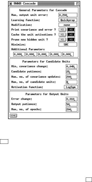
The cascade correlation control panel and the cascade window (see g. 9.3), is opened by clicking the Cascade button in the manager panel. The cascade window is needed to set the parameters of the CC learning algorithm. To start Cascade Correlation, learning function CC, update function CC Order and init function CC Weights in the corresponding menus have to be selected. If one of these functions is left out, a con rmer window with an error message pops up and learning does not start. The init functions of cascade di er from the normal init functions: upon initialization of a cascade net all hidden units are deleted.
The cascade window has the following text elds, buttons and menus:
Global parameters:
{Max. output unit error:
This value is used as abort condition for the CC learning algorithm. If the error of every single output unit is smaller than the given value learning will be terminated.
{Learning function:
Here, the learning function used to maximize the covariance or to minimize the net error can be selected from a pull down menu. Available learning functions are: Quickprop, Rprop Backprop and Batch-Backprop.
{Modification:
One of the modi cations described in the chapters 9.9.2.1 to 9.9.2.6 can be chosen. Default is no modi cation.
{Print covariance and error:
If the YES button is on, the development of the error and and the covariance of every candidate unit is printed. NO prevents all outputs of the cascade steps.
4The candidate units are realized as special units in SNNS.
9.9. THE CASCADE CORRELATION ALGORITHMS |
167 |
Figure 9.3: The cascade window
{Cache the unit activations:
If the YES button is on, the activation of a hidden unit is only calculated one time in a learning cycle. The activations are written to memory, so the next time the activation is needed, it only has to be reload. This makes CC (or TACOMA) much faster, especially for large and deep nets. On the other hand,
if the pattern set is big, too much memory (Caching needs np (ni + nh) bytes, np no of pattern, ni no of input units, nh no of hidden units) will be used. In this case you better switch caching o .
{Prune new hidden unit:
This enables \Pruned-Cascade-Correlation". It defaults to NO , which means do not remove any weights from the new inserted hidden unit. In TACOMA this button has no function.
{Minimize:
The selection criterion according to which PCC tries to minimize. The default selection criterion is the \Schwarz's Bayesian criterion", other criteria available are \Akaikes information criterion" and the \conservative mean square error of

168 |
CHAPTER 9. NEURAL NETWORK MODELS AND FUNCTIONS |
prediction". This option is ignored, unless PCC is enabled.
{Additional Parameters:
The additional values needed by TACOMA or modi ed CC. See table 9.2 for explicit information.
Candidate Parameters:
{Min. covariance change:
The covariance must change by at least this fraction of its old value to count as a signi cant change. If this fraction is not reached, learning is halted and the candidate unit with the maximum covariance is changed into a hidden unit.
{Candidate patience:
After this number of steps the program tests whether there is a signi cant change of the covariance. The change is said to be signi cant if it is larger than the fraction given by Min. covariance change.
{Max. no. of covariance updates:
The maximum number of steps to calculate the covariance. After reaching this number, the candidate unit with the maximum covariance is changed to a hidden unit.
{Max. no. of candidate units:
CC: The number of candidate units trained at once.
TACOMA: The number of points in input space within the self-organising map. As a consequence, it's the maximum number of units in the actual hidden layer.
{Activation function:
This menu item makes it possible to choose between di erent activation functions for the candidate units. The functions are: Logistic, LogSym, Tanh, Sinus, Gauss and Random. Random is not a real activation function. It randomly assigns one of the other activation functions to each candidate unit. The
function LogSym is identical to Logistic, except that it is shifted by ;0:5 along the y-axis. Sinus realizes the sin function, Gauss realizes ex2=2.
Output Parameters:
{Error change:
analogous to Min. covariance change
{Output patience:
analogous to Candidate patience
{Max. no. of epochs:
analogous to Max. no. of covariance updates
The button DELETE CAND. UNITS was deleted from this window. Now all candidates are automatically deleted at the end of training.