

Параллельные Процессы и Параллельное Программирование / SNNSv4.2.Manual
.pdf8.1. INVERSION |
139 |
as possible to the target output. There may be several input patterns generating the same output. To reduce the number of possible input patterns, the second approximation speci es a pattern the computed input pattern should approximate as well as possible. For a setting of 1.0 for the variable Input pattern the algorithm tries to keep as many input units as possible on a high activation, while a value of 0.0 increases the number of inactive input units. The variable 2nd approx ratio de nes then the importance of this input approximation.
It should be mentioned, however, that the algorithm is very unstable. One inversion run may converge, while another with only slightly changed variable settings may run inde nitely. The user therefore may have to try several combinations of variable values before a satisfying result is achieved. In general, the better the net was previously trained, the more likely is a positive inversion result.
6. HELP : Opens a window with a short help on handling the inversion display.
The network is displayed in the lower part of the window according to the settings of the last opened 2D{display window. Size, color, and orientation of the units are read from that display pointer.
8.1.3Example Session
The inversion display may be called before or after the network has been trained. A patternle for the network has to be loaded prior to calling the inversion. A target output of the network is de ned by selecting one or more units in the 2D{display by clicking the middle mouse button. After setting the variables in the setup window, the inversion run is started by clicking the start button. At regular intervals, the inversion gives a status report on the shell window, where the progress of the algorithm can be observed. When there are no more error units, the program terminates and the calculated input pattern is displayed. If the algorithm does not converge, the run can be interrupted with the stop button and the variables may be changed. The calculated pattern can be tested for correctness by selecting all input units in the 2D{display and then deselecting them immediately again. This copies the activation of the units to the display. It can then be de ned and tested with the usual buttons in the control panel. The user is advised to delete the generated pattern, since its use in subsequent learning cycles alters the behavior of the network which is generally not desirable.
Figure 8.2 shows an example of a generated input pattern (left). Here the minimum active units for recognition of the letter 'V' are given. The corresponding original pattern is shown on the right.

140 |
CHAPTER 8. NETWORK ANALYZING TOOLS |
Figure 8.2: An Example of an Inversion Display (left) and the original pattern for the letter V
8.2Network Analyzer
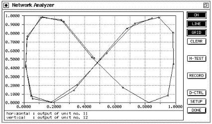
The network analyzer is a tool to visualize di erent types of graphs. An overview of these graphs is shown in table 8.1. This tool was especially developed for the prediction of time series with partial recurrent networks, but is also useful for regular feedforward networks. Its window is opened by selecting the entry ANALYZER in the menu under the GUI button.
The x-y graph is used to draw the activations or outputs of two units against each other. The t-y graph displays the activation (or output) of a unit during subsequent discrete time steps. The t-e graph makes it possible to visualize the error during subsequent discrete time steps.
Type |
Axes |
|
|
|
|
x{y |
hor.: activation or output of a unit x |
|
ver.: activation or output of a unit y |
|
|
t{y |
hor.: time t |
|
ver.: activation or output of a unit y |
t{e |
hor.: time t |
|
ver.: error e |
Table 8.1: The di erent types of graphs, which can be visualized with the network analyzer.
On the right side of the window, there are di erent buttons with the following functions:
ON : This button is used to "switch on" the network analyzer. If the Network Analyzer is switched on, every time a pattern has been propagated through the network, the network analyzer updates its display.
LINE : The points will be connected by a line, if this button is toggled.
8.2. NETWORK ANALYZER |
141 |
|
|
Figure 8.3: The Network Analyzer Window. |
|||
|
: |
Displays a grid. The number of rows and columns of the grid can be |
|||
GRID |
|||||
|
|
speci ed in the network analyzer setup. |
|||
|
: |
This button clears the graph in the display. The time counter will be |
|||
CLEAR |
|||||
|
|
reset to 1. If there is an active M--TEST operation, this operation will |
|||
|
|
be killed. |
|||
|
: |
A click on this button corresponds to several clicks on the |
|
|
button |
M-TEST |
TEST |
||||
|
|
in the control panel. The number n of TEST operations to be executed |
|||
|
|
can be speci ed in the Network Analyzer setup. Once pressed, the |
|||
|
|
button remains active until all n TEST operations have been |
executed |
||
|
|
or the M--TEST operation has been killed, e.g. by clicking the |
STOP |
||
|
|
button in the control panel. |
|||
|
: If this button activated, the points will not only be shown on the display, |
||||
RECORD |
|||||
|
|
but their coordinates will also be saved in a le. The name of this le |
|||
|
|
can be speci ed in the setup of the Network Analyzer. |
|||
|
: |
Opens the display control window of the Network Analyzer. The de- |
|||
D-CTRL |
|||||
|
|
scription of this window follows below. |
|||
|
: |
Opens the Network Analyzer setup window. The description of the |
|||
SETUP |
|||||
|
|
setup follows in the next subsection. |
|||
|
: |
Closes the network analyzer window. An active M--TEST operation will |
|||
DONE |
|||||
|
|
be killed. |
|||

142 |
CHAPTER 8. NETWORK ANALYZING TOOLS |
8.2.1The Network Analyzer Setup
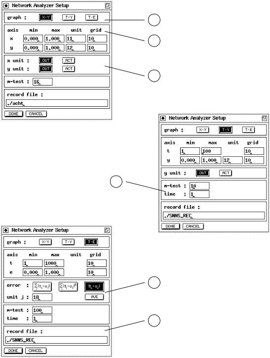
The setup window can be opened by pressing the SETUP button on the right side of the network analyzer window. The shape of the setup window depends on the type of graph to display (see g. 8.4).
The setup window consists of ve parts (see g. 8.4):
1To select the type of graph (see table 8.1) to be displayed, press the corresponding button X-Y , T-Y or T-E .
2The second part of the setup window is used to specify some attributes about the axes. The rst line contains the values for the axes in horizontal direction, the second line these for the vertical axes. The columns min and max de ne the area to be displayed. The numbers of the units, whose activation or output values should be drawn have to be speci ed in the column unit. The last column grid the number of columns and rows of the grid can be varied. The labeling of the axes is dependent on these values, too.
3a |
The selection between showing the activation or the output of a unit along the x{ |
|||||||||||||
or y{axes can be made here. To draw the output of a unit click on |
OUT |
and to |
||||||||||||
|
||||||||||||||
|
draw the activation of a unit click on |
ACT |
. |
|
|
|||||||||
3b |
Di erent types of error curves can be drawn: |
|||||||||||||
|
|
|
|
|
|
|
|
|
|
|
|
|
||
|
|
|
For each output unit the di erence between the generated |
|||||||||||
|
i jti ; oij |
|
||||||||||||
|
|
output and the teaching output is computed. The error is |
||||||||||||
|
X |
|
computed as the sum of the absolute values of the di erences. |
|||||||||||
|
|
|
||||||||||||
|
|
|
If |
AVE |
is toggled, the result is divided by the number of |
|||||||||
|
|
|
output units, giving the average error per output unit. |
|||||||||||
|
|
|
The error is computed as above, but the square of the di er- |
|||||||||||
|
i jti ; oij2 |
|
||||||||||||
|
|
ences is taken instead of the absolute values. With |
AVE |
the |
||||||||||
|
X |
|
|
|
|
|
|
|||||||
|
|
mean squared deviation is computed. |
||||||||||||
|
|
|
||||||||||||
|
|
|
Here the deviation of only a single output unit is processed. |
|||||||||||
|
jtj ; ojj |
|
||||||||||||
|
|
The number of the unit is speci ed as unit j. |
||||||||||||
4 |
m-test: |
Speci es the number of TEST operations, which have to be executed |
||||||||||||
|
when clicking on |
M-TEST |
button. |
|||||||||||
|
|
|||||||||||||
|
time: |
Sets the time counter to the given value. |
||||||||||||
5The name of the le, in which the visualized data can be saved by activating the RECORD button, can be speci ed here. The lename will be automatically extended by the su x '.rec'. To change the lename, the RECORD button must not be activated.
8.2. NETWORK ANALYZER |
143 |
y
y
1
2
3a
4
z
3b
9
5
9
Figure 8.4: The Network Analyzer SetupWindows: the setup window for a x-y{graph (top), the setup window for a t-y{graph (middle) and the setup window for a t-e{graph (bottom).
144 |
CHAPTER 8. NETWORK ANALYZING TOOLS |
When the setup is left by clicking on CANCEL When leaving the setup by pressing the DONE errors could be detected.
all the changes made in the setup are lost. button, the changes will be accepted if no
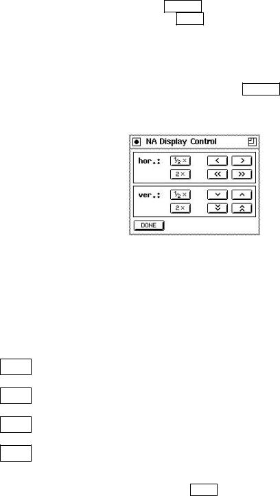
8.2.2The Display Control Window of the Network Analyzer
The display control window appears, when clicking on D-CTRL button on the right side of the network analyzer window. This windows is used to easily change the area in the display of the network analyzer.
Figure 8.5: The display control window of the network analyzer
The buttons to change the range of the displayed area in horizontal direction have the following functions:
1=2 |
: |
The length of the interval is to be bisected. The lower bound remains. |
|
|
|
2 |
: |
The length of the interval is to be doubled. The lower bound remains. |
<: Shifts the range to the left by the width of a grid column.
>: Shifts the range to the right by the width of a grid column.
: Shifts the range to the left by the length of the interval.
: Shifts the range to the right by the length of the interval.
The buttons to change the range in vertical direction have a corresponding function. To close the display control window, press the DONE button.
Chapter 9
Neural Network Models and
Functions
The following chapter introduces the models and learning functions implemented in SNNS. A strong emphasis is placed on the models that are less well known. They can not, however, be explained exhaustively here. We refer interested users to the literature.
9.1Backpropagation Networks
9.1.1Vanilla Backpropagation
The standard backpropagation learning algorithm introduced by [RM86] and described already in section 3.3 is implemented in SNNS. It is the most common learning algorithm. Its de nition reads as follows:
wij |
= |
j |
oi |
|
j |
= |
fj0 |
(netj)(tj ; oj) |
if unit j is an output unit |
|
|
( fj0 |
(netj) Pk kwjk |
if unit j is a hidden unit |
This algorithm is also called online backpropagation because it updates the weights after every training pattern.
9.1.2Enhanced Backpropagation
An enhanced version of backpropagation uses a momentum term and at spot elimination. It is listed among the SNNS learning functions as BackpropMomentum.
The momentum term introduces the old weight change as a parameter for the computation of the new weight change. This avoids oscillation problems common with the regular
146 |
CHAPTER 9. NEURAL NETWORK MODELS AND FUNCTIONS |
backpropagation algorithm when the error surface has a very narrow minimum area. The new weight change is computed by
wij(t + 1) = j oi + wij (t)is a constant specifying the in uence of the momentum.
The e ect of these enhancements is that at spots of the error surface are traversed relatively rapidly with a few big steps, while the step size is decreased as the surface gets rougher. This adaption of the step size increases learning speed signi cantly.
Note that the old weight change is lost every time the parameters are modi ed, new patterns are loaded, or the network is modi ed.
9.1.3Batch Backpropagation
Batch backpropagation has a similar formula as vanilla backpropagation. The di erence lies in the time when the update of the links takes place. While in vanilla backpropagation an update step is performed after each single pattern, in batch backpropagation all weight changes are summed over a full presentation of all training patterns (one epoch). Only then, an update with the accumulated weight changes is performed. This update behavior is especially well suited for training pattern parallel implementations where communication costs are critical.
9.1.4Backpropagation with chunkwise update
There is a third form of Backpropagation, that comes in between the online and batch versions with regard to updating the weights. Here, a chunk is de ned as the number of patterns to be presented to the network before making any alternations to the weights. This version is very useful for training cases with very large training sets, where batch update would take to long to converge and online update would be too instable. We found to achieve excellent results with chunk sizes between 10 and 100 patterns.
This algorithm allows also to add random noise to the link weights before the handling of each chunk. This weights jogging proofed to be very useful for complicated training tasks. Note, however, that it has to be used very carefully! Since this noise is added fairly frequently, it can destroy all learning progress if the noise limits are chosen to large. We recommend to start with very small values (e.g. [-0.01 , 0.01]) and try larger values only when everything is looking stable. Note also, that this weights jogging is independent from the one de ned in the jog-weights panel. If weights jogging is activated in the jog-weights panel, it will operate concurrently, but on an epoch basis and not on a chunk basis. See section 4.3.3 for details on how weights jogging is performed in SNNS.
It should be clear, that weights jogging will make it hard to reproduce your exact learning results!
Another new feature introduced by this learning scheme is the notion of selective updating of units. This feature can be exploited only with patterns that contain class information. See chapter 5.4 for details on this pattern type.

9.1. BACKPROPAGATION NETWORKS |
147 |
Using class based pattern sets and a special naming convention for the network units, this learning algorithm is able to train di erent parts of the network individually. Given the example pattern set of page 98, it is possible to design a network which includes units that are only trained for class A or for class B (independent of whether additional class redistribution is active or not). To utilise this feature the following points must be observed.
Within this learning algorithm, di erent classes are known by the number of their position according to an alphabetic ordering and not by their class names. E.g.: If there are pattern classes named alpha, beta, delta, all alpha patterns belong to class number 0, all beta patterns to number 1, and all delta patterns to class number 2.
If the name of a unit matches the regular expression class+x[+y]* (x,y 2 f0 1 :::32g), it is trained only if the class number of the current pattern matches one of the given x, y, ... values. E.g.: A unit named class+2 is only trained on patterns with class number 2, a unit named class+2+0 is only trained on patterns with class number 0 or 2.
If the name of a unit matches the regular expression class-x[-y]* (x,y 2 f0 1 :::32g), it is trained only if the the class number of the current pattern does not match any of the given x, y, ... values. E.g.: A unit named class-2 is trained on all patterns but those with class number 2, a unit named class-2-0 is only trained on patterns with class numbers other than 0 and 2.
All other network units are trained as usual.
The notion of training or not training a unit in the above description refers to adding up weight changes for incoming links and the unit's bias value. After one chunk has been completed, each link weight is individually trained (or not), based on its own update count. The learning rate is normalised accordingly.
The parameters this function requires are:
: learning parameter, speci es the step width of the gradient descent as with Std Backpropagation. Use the same values as there (0.2 to 0.5).
dmax: the maximum training output di erences as with Std Backpropagation. Usually set to 0.0
N: chunk size. The number of patterns to be presented during training before an update of the weights with the accumulated error will take place. Depending on the overall size of the pattern set used, a value between 10 and 100 is suggested here.
lowerlimit: Lower limit for the range of random noise to be added for each chunk.
upperlimit: Upper limit for the range of random noise to be added for each chunk. If both upper and lower limit are 0.0, no weights jogging takes place.

148 |
CHAPTER 9. NEURAL NETWORK MODELS AND FUNCTIONS |
9.1.5Backpropagation with Weight Decay
Weight Decay was introduced by P. Werbos ([Wer88]). It decreases the weights of the links while training them with backpropagation. In addition to each update of a weight by backpropagation, the weight is decreased by a part d of its old value. The resulting formula is
wij(t + 1) = j oi ; d wij(t)
The e ect is similar to the pruning algorithms (see chapter 10). Weights are driven to zero unless reinforced by backpropagation. For further information, see [Sch94].
9.2Quickprop
One method to speed up the learning is to use information about the curvature of the error surface. This requires the computation of the second order derivatives of the error function. Quickprop assumes the error surface to be locally quadratic and attempts to jump in one step from the current position directly into the minimum of the parabola.
Quickprop [Fah88] computes the derivatives in the direction of each weight. After computing the rst gradient with regular backpropagation, a direct step to the error minimum is attempted by
S(t + 1)
(t + 1)wij = S(t) ; S(t + 1) (t)wij
where:
wij weight between units i and j(t + 1) actual weight change
S(t + 1) partial derivative of the error function by wij S(t) the last partial derivative
9.3RPROP
9.3.1Changes in Release 3.3
The implementation of Rprop has been changed in two ways: First, the implementation now follows a slightly modi ed adaptation scheme. Essentially, the backtracking step is no longer performed, if a jump over a minimum occurred. Second, a weight-decay term is introduced. The weight-decay parameter (the third learning parameter) determines the relationship of two goals, namely to reduce the output error (the standard goal) and to reduce the size of the weights (to improve generalization). The composite error function is:
E = X(ti ; oi)2 + 10; Xwij2