

Параллельные Процессы и Параллельное Программирование / SNNSv4.2.Manual
.pdf7.2. BIGNET FOR TIME-DELAY NETWORKS |
129 |
||||||||||
|
|
|
|
|
|
|
|
|
|
|
|
|
|
|
|
|
|
|
|
|
|
|
|
|
|
|
|
|
|
|
|
|
|
|
|
|
|
|
|
|
|
|
|
|
|
|
|
Figure 7.11: An example TDNN construction and the resulting network
The first feature unit |
The first feature unit |
|
for hidden unit 2 |
||
for hidden unit 1 |
||
|
Input Layer |
Hidden Layer |
Figure 7.12: Two receptive elds in one layer
It is possible to specify seperate receptive elds for di erent feature units. With only one receptive eld for all feature units, a "1" has to be speci ed in the input window for "1st feature unit:". For a second receptive eld, the rst feature unit should be the width of
130 |
CHAPTER 7. GRAPHICAL NETWORK CREATION TOOLS |
the rst receptive eld plus one. Of course, for all number of receptive elds, the sum of their width has to equal the number of feature units! An example network with two receptive elds is depicted in gure 7.12
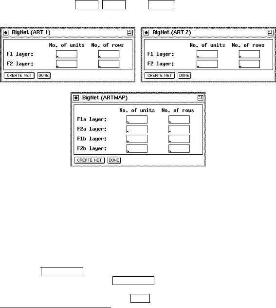
7.3BigNet for ART-Networks
The creation of the ART networks is based on just a few parameters. Although the network topology for these models is rather complex, only four parameters for ART1 and ART2, and eight parameters for ARTMAP, have to be speci ed.
If you have selected the ART 1 , ART 2 or the ARTMAP button in the BigNet menu, one of the windows shown in gure 7.13 appears on the screen.
Figure 7.13: The BigNet windows for the ART models
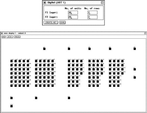
The four parameters you have to specify for ART1 and ART2 are simple to choose. First you have to tell BigNet the number of units (N) the F1 layer consists of. Since the F0 layer has the same number of units, BigNet takes only the value for F1.
Next the way how these N units to be displayed has to be speci ed. For this purpose enter the number of rows. An example for ART1 is shown in gure 7.14.
The same procedure is to be done for the F2 layer. Again you have to specify the number of units M for the recognition part1 of the F2 layer and the number of rows.
Pressing the CREATE NET button will generate a network with the speci ed parameters.
If a network exists when pressing CREATE NET you will be prompted to assure that you really want to destroy the current network. A message tells you if the generation terminated successfully. Finally press the DONE button to close the BigNet panel.
1The F2 layer consists of three internal layers. See chapter 9.13.
7.4. BIGNET FOR SELF-ORGANIZING MAPS |
131 |
Figure 7.14: Example for the generation of an ART1 network. First the BigNet (ART1) panel is shown with the speci ed parameters. Next you see the created net as you can see it when using an SNNS display.
For ARTMAP things are slightly di erent. Since an ARTMAP network exists of two ART1 subnets (ARTa and ARTb), for both of them the parameters described above have to be speci ed. This is the reason, why BigNet (ARTMAP) takes eight instead of four parameters. For the MAP eld the number of units and the number of rows is taken from the repective values for the F2b layer.
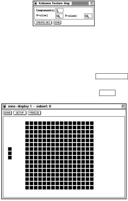
7.4BigNet for Self-Organizing Maps
As described in chapter 9.14, it is recommended to create Kohonen-Self-Organizing Maps only by using either the BigNet network creation tool or convert2snns outside the graphical user interface. The SOM architecture consists of the component layer (input layer) and a two-dimensional map, called competitive layer. Since component layer and competitive layer are fully connected, each unit of the competitive layer represents a vector with the same dimension as the component layer.
To create a SOM, only 3 parameters have to be speci ed:
Components:units. The dimension of each weight vector. It equals the number of input
132 |
CHAPTER 7. GRAPHICAL NETWORK CREATION TOOLS |
Figure 7.15: The BigNet window for the SOM architecture
X-size: The width of the competitive layer. When learning is performed, the x-size value must be speci ed by the fth learning parameter.
Y-size: The length of the competitive layer. The number of hidden (competitive) units equals X-size Y-size.
If the parameters are correct (positive integers), pressing the CREATE NET button will create the speci ed network. If the creation of the network was successful a con rming message is issued. The parameters of the above example would create the network ofgure 7.16. Eventually close the BigNet panel by pressing the DONE button.
Figure 7.16: An Example SOM
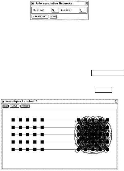
7.5BigNet for Autoassociative Memory Networks
The easiest way to create an autoassociative memory network is with the help of this bignet panel, although this type of network may also be constructed interactively with the graphical network editor. The architecture consists of the world layer (input layer) and a layer of hidden units, identical in size and shape to the world layer, called learning layer.
7.6. BIGNET FOR PARTIAL RECURRENT NETWORKS |
133 |
Each unit of the world layer has a link to the corresponding unit in the learning layer. The learning layer is connected as a clique.
Figure 7.17: The BigNet Window for Autoassociative Memory Networks
To create an autoassociative memory, only 2 parameters have to be speci ed:
X-size: The width of the world and learning layers.
Y-size: The length of the world and learning layers. The number of units in the network equals 2 X-size Y-size.
If the parameters are correct (positive integers), pressing the CREATE NET button will create the speci ed network. If the creation of the network was successful a con rming message is issued. The parameters of the above example would create the network ofgure 7.18. Eventually close the BigNet panel by pressing the DONE button.
Figure 7.18: An Example Autoassociative Memory
7.6BigNet for Partial Recurrent Networks
7.6.1BigNet for Jordan Networks
The BigNet window for Jordan networks is shown in gure 7.19.
In the column No. of Units the number of units in the input, hidden and output layer have to be speci ed. The number of context units equals the number of output units. The units of a layer are displayed in several columns. The number of these columns is given

134 |
CHAPTER 7. GRAPHICAL NETWORK CREATION TOOLS |
Figure 7.19: The BigNet Window for Jordan Networks
by the value in the column No. of Col.. The network will be generated by pressing the
CREATE NET button:
The input layer is fully connected to the hidden layer,i.e. every input unit is connected to every unit of the hidden layer. The hidden layer is fully connected to the output layer.
Output units are connected to context units by recurrent 1-to-1-connections. Every context unit is connected to itself and to every hidden unit.
Default activation function for input and context units is the identity function, for hidden and output units the logistic function.
Default output function for all units is the identity function
To close the BigNet window for Jordan networks click on the DONE button.
7.6.2BigNet for Elman Networks
By clicking on the ELMAN button in the BigNet menu, the BigNet window for Elman networks (see g.7.20) is opened.
Figure 7.20: The BigNet Window for Elman Networks
The number of units of each layer has to be speci ed in the column No. of Units. Each hidden layer is assigned a context layer having the same size. The values in the column

7.6. BIGNET FOR PARTIAL RECURRENT NETWORKS |
135 |
No. of Col. have the same meaning as the corresponding values in the BigNet window for Jordan networks.
The number of hidden layers can be changed |
with the buttons |
INSERT |
and |
DELETE |
. |
|
INSERT |
adds a new hidden layer just before |
the output layer. |
The hidden layer with |
|||
the highest layer number can be deleted by pressing the DELETE button. The current
implementation requires at least one and at most eight hidden layers. If the network is supposed to also contain a context layer for the output layer, the YES button has to be toggled, else the NO button. Press the CREATE NET button to create the net. The generated network has the following properties:
The layer i is fully connected to the layer i + 1.
Each context layer is fully connected to its hidden layer. A hidden layer is connected to its context layer with recurrent 1-to-1-connections.
Each context unit is connected to itself.
If there is a context layer assigned to the output layer, the same connection rules as for hidden layers are used.
Default activation function for input and context units is the identity function, for hidden and output units the logistic function.
Default output function for all units is the identity function
Click on the DONE button to close the BigNet window for Elman networks.
Chapter 8
Network Analyzing Tools
8.1Inversion
Very often the user of a neural network asks what properties an input pattern must have in order to let the net generate a speci c output. To help answer this question, the Inversion algorithm developed by J. Kindermann and A. Linden ([KL90]) was implemented in SNNS.
8.1.1The Algorithm
The inversion of a neural net tries to nd an input pattern that generates a speci c output pattern with the existing connections. To nd this input, the deviation of each output from the desired output is computed as error . This error value is used to approach the target input in input space step by step. Direction and length of this movement is computed by the inversion algorithm.
The most commonly used error value is the Least Mean Square Error. ELMS is de ned as
n
ELMS = |
[Tp ; f( wijopi)]2 |
p=1 |
i |
X |
X |
The goal of the algorithm therefore has to be to minimize ELMS.
Since the error signal pi can be computed as
2 X |
|
|
pi = opi(1 ; opi) |
|
pkwik |
k |
Succ(i) |
|
and for the adaption value of the unit activation follows
4netpi = pi resp. netpi = netpi + pi
8.1. INVERSION |
137 |
In this implementation, a uniform pattern is applied to the input units in the rst step, whose activation level depends upon the variable input pattern. This pattern is propagated through the net and generates the initial output O(0). The di erence between this output vector and the target output vector is propagated backwards through the net as error signals i(0) . This is analogous to the propagation of error signals in the backpropagation training, with the di erence that no weights are adjusted here. When the error signals reach the input layer, they represent a gradient in input space, which gives the direction for the gradient descent. Thereby, the new input vector can be computed as
I(1) = I(0) + i(0)
where is the step size in input space, which is set by the variable eta.
This procedure is now repeated with the new input vector until the distance between the generated output vector and the desired output vector falls below the prede ned limit of delta max, when the algorithm is halted.
For a more detailed description of the algorithm and its implementation see [Mam92].
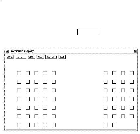
8.1.2Inversion Display
The inversion algorithm is called by clicking the INVERSION button in the manager panel.
Picture 8.1 shows an example of the generated display.
Figure 8.1: The Inversion Display
The display consists of two regions. The larger, lower part contains a sketch of the input and output units of the network, while the upper line holds a series of buttons. Their respective functions are:
138 |
CHAPTER 8. NETWORK ANALYZING TOOLS |
1.DONE : Quits the inversion algorithm and closes the display.
2.STEP : Starts / Continues the algorithm. The program starts iterating by slowly changing the input pattern until either the STOP button is pressed, or the generated output pattern approximates the desired output pattern su ciently well. Su ciently well means that all output units have an activation which di ers from the expected
activation of that unit by at most a value of max. This error limit can be set in the setup panel (see below). During the iteration run, the program prints status reports to stdout.
cycle 50 inversion error 0.499689 still 1 error unit(s) cycle 100 inversion error 0.499682 still 1 error unit(s) cycle 150 inversion error 0.499663 still 1 error unit(s) cycle 200 inversion error 0.499592 still 1 error unit(s) cycle 250 inversion error 0.499044 still 1 error unit(s) cycle 269 inversion error 0.000000 0 error units left
where cycle is the number of the current iteration, inversion error is the sum of the squared error of the output units for the current input pattern, and error units are all units that have an activation that di ers more than the value of max from the target activation.
3. STOP : Interrupts the iteration. The status of the network remains unchanged. The interrupt causes the current activations of the units to be displayed on the screen. A click to the STEP button continues the algorithm from its last state. Alternatively
the algorithm can be reset before the restart by a click to the NEW button, or continued with other parameters after a change in the setup. Since there is no automatic recognition of in nite loops in the implementation, the STOP button is also necessary when the algorithm obviously does not converge.
4.NEW Resets the network to a de ned initial status. All variables are assigned the values in the setup panel. The iteration counter is set to zero.
5.SETUP : Opens a pop-up window to set all variables associated with the inversion. These variables are:
eta |
The step size for changing the activations. It should range |
||||
|
|
|
from 1.0 to 10.0. Corresponds to the learning factor in |
||
|
|
|
backpropagation. |
||
delta |
|
max |
The maximum activation deviation of an output unit. |
||
|
|||||
|
|
|
Units with higher deviation are called error units. |
||
|
|
|
A typical value of delta |
|
max is 0.1. |
|
|
|
|
||
Input pattern |
Initial activation of all input units. |
||||
2nd approx ratio |
In uence of the second approximation. Good values range |
||||
|
|
|
from 0.2 to 0.8. |
||
A short description of all these variables can be found in an associated help window, which pops up on pressing HELP in the setup window.
The variable second approximation can be understood as follows: Since the goal is to get a desired output, the rst approximation is to get the network output as close