Analyzing the Texture of an Image

Gray-Level Co-Occurrence Matrix (GLCM)

A statistical method of examining texture that considers the spatial relationship of pixels is the gray-level co-occurrence matrix (GLCM), also known as the gray-level spatial dependence matrix. The GLCM functions characterize the texture of an image by calculating how often pairs of pixel with specific values and in a specified spatial relationship occur in an image, creating a GLCM, and then extracting statistical measures from this matrix. (The texture filter functions, described in “Using Texture Filter Functions” on page 11-27, cannot provide information about shape, i.e., the spatial relationships of pixels in an image.)

After you create the GLCMs, you can derive several statistics from them using the graycoprops function. These statistics provide information about the texture of an image. The following table lists the statistics.

Create a Gray-Level Co-Occurrence Matrix

To create a GLCM, use the graycomatrix function. The graycomatrix function creates a gray-level co-occurrence matrix (GLCM) by calculating how often a pixel with the intensity (gray-level) value i occurs in a specific spatial relationship to a pixel with the value j. By default, the spatial relationship is defined as the pixel of interest and the pixel to its immediate right (horizontally adjacent), but you can specify other spatial relationships between the two pixels. Each element (i,j) in the resultant glcm is simply the sum of the number of times that the pixel with value i occurred in the specified spatial relationship to a pixel with value j in the input image.

11-31

11 Analyzing and Enhancing Images

The number of gray levels in the image determines the size of the GLCM. By default, graycomatrix uses scaling to reduce the number of intensity values in an image to eight, but you can use the NumLevels and the GrayLimits parameters to control this scaling of gray levels. See the graycomatrix reference page for more information.

The gray-level co-occurrence matrix can reveal certain properties about the spatial distribution of the gray levels in the texture image. For example, if most of the entries in the GLCM are concentrated along the diagonal, the texture is coarse with respect to the specified offset. You can also derive several statistical measures from the GLCM. See for more information.

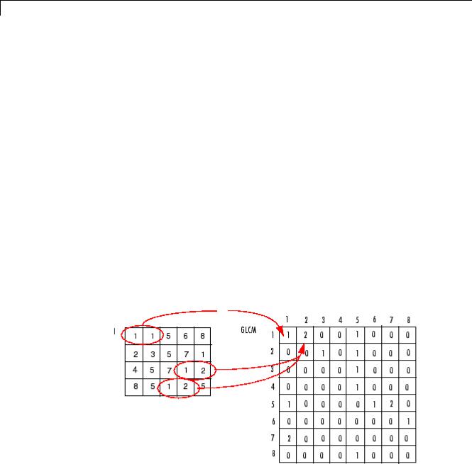
To illustrate, the following figure shows how graycomatrix calculates the first three values in a GLCM. In the output GLCM, element (1,1) contains the value 1 because there is only one instance in the input image where two horizontally adjacent pixels have the values 1 and 1, respectively. glcm(1,2) contains the value 2 because there are two instances where two horizontally adjacent pixels have the values 1 and 2. Element (1,3) in the GLCM has the value 0 because there are no instances of two horizontally adjacent pixels with the values 1 and 3. graycomatrix continues processing the input image, scanning the image for other pixel pairs (i,j) and recording the sums in the corresponding elements of the GLCM.

Process Used to Create the GLCM

11-32

Analyzing the Texture of an Image

Specifying the Offsets

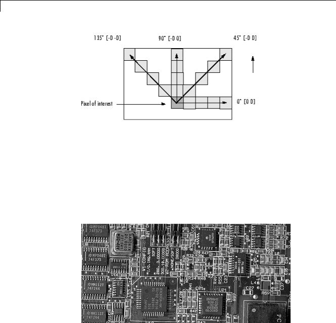
By default, the graycomatrix function creates a single GLCM, with the spatial relationship, or offset, defined as two horizontally adjacent pixels. However, a single GLCM might not be enough to describe the textural features of the input image. For example, a single horizontal offset might not be sensitive to texture with a vertical orientation. For this reason, graycomatrix can create multiple GLCMs for a single input image.

To create multiple GLCMs, specify an array of offsets to the graycomatrix function. These offsets define pixel relationships of varying direction and distance. For example, you can define an array of offsets that specify four directions (horizontal, vertical, and two diagonals) and four distances. In this case, the input image is represented by 16 GLCMs. When you calculate statistics from these GLCMs, you can take the average.

You specify these offsets as a p-by-2 array of integers. Each row in the array is a two-element vector, [row_offset, col_offset], that specifies one offset. row_offset is the number of rows between the pixel of interest and its neighbor. col_offset is the number of columns between the pixel of interest and its neighbor. This example creates an offset that specifies four directions and 4 distances for each direction. For more information about specifying offsets, see the graycomatrix reference page.

The figure illustrates the spatial relationships of pixels that are defined by this array of offsets, where D represents the distance from the pixel of interest.

11-33

11 Analyzing and Enhancing Images

Derive Statistics from a GLCM and Plot Correlation

This example shows how to create a set of GLCMs and derive statistics from them and illustrates how the statistics returned by graycoprops have a direct relationship to the original input image.

1Read in a grayscale image and display it. The example converts the truecolor image to a grayscale image and then rotates it 90° for this example.

circuitBoard = rot90(rgb2gray(imread('board.tif'))); imshow(circuitBoard)

11-34

Analyzing the Texture of an Image

2Define offsets of varying direction and distance. Because the image contains objects of a variety of shapes and sizes that are arranged in horizontal and vertical directions, the example specifies a set of horizontal offsets that only vary in distance.

offsets0 = [zeros(40,1) (1:40)'];

3Create the GLCMs. Call the graycomatrix function specifying the offsets. glcms = graycomatrix(circuitBoard,'Offset',offsets0)

4Derive statistics from the GLCMs using the graycoprops function. The example calculates the contrast and correlation.

stats = graycoprops(glcms,'Contrast Correlation');

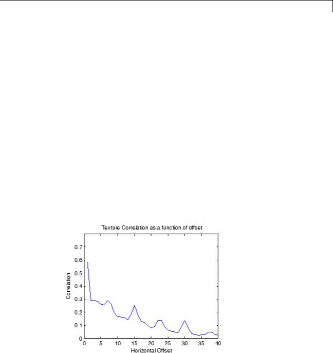
5Plot correlation as a function of offset.

figure, plot([stats.Correlation]);

title('Texture Correlation as a function of offset'); xlabel('Horizontal Offset')

ylabel('Correlation')

11-35

11 Analyzing and Enhancing Images

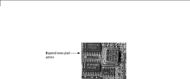
The plot contains peaks at offsets 7, 15, 23, and 30. If you examine the input image closely, you can see that certain vertical elements in the image have a periodic pattern that repeats every seven pixels. The following figure shows the upper left corner of the image and points out where this pattern occurs.

11-36