Radon Transform

Radon Transform

In this section...

“Radon Transformation Definition” on page 9-19 “Plotting the Radon Transform” on page 9-22

“Viewing the Radon Transform as an Image” on page 9-24 “Detecting Lines Using the Radon Transform” on page 9-25

Note For information about creating projection data from line integrals along paths that radiate from a single source, called fan-beam projections, see “Fan-Beam Projection Data” on page 9-36. To convert parallel-beam projection data to fan-beam projection data, use the para2fan function.

Radon Transformation Definition

The radon function computes projections of an image matrix along specified directions.

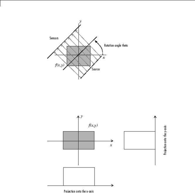
A projection of a two-dimensional function f(x,y) is a set of line integrals. The radon function computes the line integrals from multiple sources along parallel paths, or beams, in a certain direction. The beams are spaced 1 pixel unit apart. To represent an image, the radon function takes multiple, parallel-beam projections of the image from different angles by rotating the source around the center of the image. The following figure shows a single projection at a specified rotation angle.

9-19

9 Transforms

Parallel-Beam Projection at Rotation Angle Theta

For example, the line integral of f(x,y) in the vertical direction is the projection of f(x,y) onto the x-axis; the line integral in the horizontal direction is the projection of f(x,y) onto the y-axis. The following figure shows horizontal and vertical projections for a simple two-dimensional function.

Horizontal and Vertical Projections of a Simple Function

9-20

Radon Transform

Projections can be computed along any angle [[THETA]]. In general, the Radon transform of f(x,y) is the line integral of f parallel to the y´-axis

The following figure illustrates the geometry of the Radon transform.

Geometry of the Radon Transform

9-21

9 Transforms

Plotting the Radon Transform

You can compute the Radon transform of an image I for the angles specified in the vector theta using the radon function with this syntax.

[R,xp] = radon(I,theta);

The columns of R contain the Radon transform for each angle in theta. The vector xp contains the corresponding coordinates along the x′-axis. The center pixel of I is defined to be floor((size(I)+1)/2); this is the pixel on the

x′-axis corresponding to x′ = 0 .

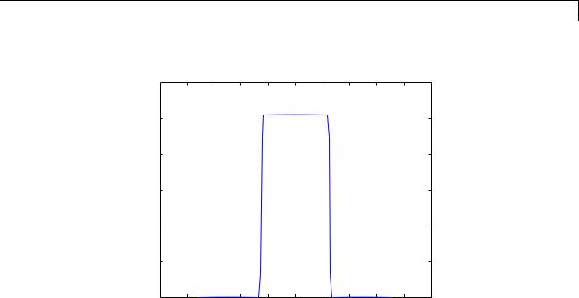
The commands below compute and plot the Radon transform at 0° and 45° of an image containing a single square object. xp is the same for all projection angles.

I = zeros(100,100); I(25:75, 25:75) = 1; imshow(I)

[R,xp] = radon(I,[0 45]);

figure; plot(xp,R(:,1)); title('R_{0^o} (x\prime)')

9-22

Radon Transform

R0o (x′)

Radon Transform of a Square Function at 0 Degrees figure; plot(xp,R(:,2)); title('R_{45^o} (x\prime)')

9-23