output gain control. These parameters directly or indirectly modify the variables m, c, k1, and k3. To simplify the effect’s tuning k = k1 = k3 is called the nonlinearity parameter. This condition fixes the stable positions of the system respectively at x = −1 and x = 1. Therefore, by increasing the nonlinearity parameter, the slope of the polynomial curve increases as well as the amount of excitation amplitude required to move across the stable positions.

The resonance frequency parameter allows to adjust the system’s resonance frequency, changing the pitch of the sound effect. With the two parameters mentioned previously, the value for the mass is computed from Eq. (2) using only the linear part of the stiffness k = k1 assuming small displacements of the mass to simplify the problem.

A damping parameter is included to control the amount of interwell and intrawell oscillations. Increasing this parameter will reduce sustaining oscillations of the effect and can even restrict the mass from going through a snapthrough.

The final algorithm is adjusted for input and output signal levels. The input signal f[n], being a digital signal with values between −1 and 1 is adjustable by the variable input Gain Control. The output signal x˙[n], proportional to velocity is first divided by 104 to get the output values near the values corresponding to a digital signal between −1 and 1, and then adjusted by the variable output Gain Control.

3.4. VST Plugin and Online Demo Application

To provide a possibility to play and listen the effect, we built two applications. The fist one is a VST plugin, the second one is an online web-audio application. Both are using the same parameters as the ones described above.

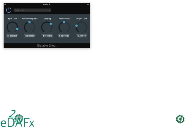
The VST plugin is implemented using the JUCE Framework [25]. The source code, as well as compiled versions for MacOSX and Windows, are available online at https://ant-novak. com/bistable_effect [21]. A print-screen of the final VTS plugin is shown in Fig. 14.

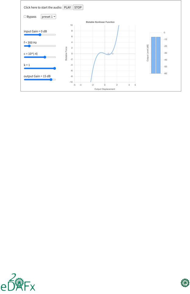
circles added to this graph show the real-time envelope (maximum and minimum) of the output displacement.

4. CONCLUSION

This work was a part of the master student project in the frame of the International Master’s Degree in Electro-Acoustics (IMDEA) program at the Le Mans University (France). Its goal was to implement a bistable system, a system well known from nonlinear dynamics and vibrations research, as a digital audio effect.

Bistability in systems is a complex subject to model and analyze, let alone, to successfully implement its principle into an audio effect. On the other hand, the sounds obtained by this approach are unique and rewarding, leaving a big window for future research and development on the usage of these systems to develop sound effects.

Even though the model is simple to write and implement, achieving a pleasant sound that could be used for sound effects is not an easy task. Indeed, it is crucial to fully understand the operation points of this system to fine-tune its parameters and get the most out of this particular system. For this, the force-displacement curve gives the best insight into how the system performs.

Due to the presence of co-existing steady-state dynamics, the output of a bistable system is different each time, even though the same excitation parameters are used. The bistable effect has no unique sound, but a wide variety of different sounds that depend on the combination of its parameters.

Future work will be focused on application of more sophisticated difference scheme such as energy-consistent numerical methods ([27]) or application of port-Hamiltonian approach [10]), and the accuracy of the discretized bistable system in comparison with the original continuous-time system.

5. ACKNOWLEDGMENTS

This paper is a result of the master student project in the frame of the International Master’s Degree in Electro-Acoustics (IMDEA) program at the Le Mans University (France). The students Alexander Ramirez and Vikas Tokala contributed equally to all parts of the project including project management, measurement, coding the VST plugin, building the mechanical prototype, and writing of the paper. Antonin Novak, Frederic Ablitzer, and Manuel Melon only supervised the project and helped with the review process. The web-audio JavaScript applet was written by Antonin Novak based on the C++ code provided by the students.

6. REFERENCES

Figure 14: Bistable Plugin User Guide Interface.

The online web demo application of the bistable audio effect developed using the Web Audio API [26] is available at https://ant-novak.com/bistable_effect [21]. Its print screen is shown in Fig. 15. The input signal is a short loop of a guitar sample. Several presets are available to select different configurations. Another part of the demo application is a graph that shows the shape of the nonlinear bistable curve to visualize in real-time the state of the displacement-force relation. The two grey

DAFx.6

114

[1]U. Zölzer, DAFX:Digital Audio Effects, John Wiley & Sons, 2002.

[2]Michael E McIntyre, Robert T Schumacher, and James Woodhouse, “On the oscillations of musical instruments,”

The Journal of the Acoustical Society of America, vol. 74, no. 5, pp. 1325–1345, 1983.

[3]Antoine Chaigne and Jean Kergomard, Acoustics of musical instruments, Springer, 2016.

[4]V Debut, J Antunes, M Marques, and M Carvalho, “Physicsbased modeling techniques of a twelve-string portuguese guitar: A non-linear time-domain computational approach

2 in21

DAFx

for the multiple-strings/bridge/soundboard coupled dynamics,” Applied acoustics, vol. 108, pp. 3–18, 2016.

[5]Clara Issanchou, Stefan Bilbao, Jean-Loic Le Carrou, Cyril Touzé, and Olivier Doaré, “A modal-based approach to the nonlinear vibration of strings against a unilateral obstacle: Simulations and experiments in the pointwise case,” Journal of Sound and Vibration, vol. 393, pp. 229–251, 2017.

[6]Insook Choi, “Sound synthesis and composition applying time scaling to observing chaotic systems.,” in Proceedings of the 2nd International Conference on Auditory Display (ICAD1994), Santa Fe, New Mexico, 1994, pp. 79–107.

[7]Antoine Chaigne, Cyril Touzé, and Olivier Thomas, “Nonlinear vibrations and chaos in gongs and cymbals,” Acoustical science and technology, vol. 26, no. 5, pp. 403–409, 2005.

[8]Antonin Novak, Laurent Simon, Pierrick Lotton, and Joël Gilbert, “Chebyshev model and synchronized swept sine method in nonlinear audio effect modeling,” in Proc. 13th Int. Conference on Digital Audio Effects (DAFx-10), 2010, p. 15.

[9]Felix Eichas, Stephan Möller, and Udo Zölzer, “Blockoriented modeling of distortion audio effects using iterative minimization,” Proc. Digital Audio Effects (DAFx-15), Trondheim, Norway, 2015.

[10]Antoine Falaize and Thomas Hélie, “Guaranteed-passive simulation of an electro-mechanical piano: A porthamiltonian approach,” in Proc. Digital Audio Effects (DAFx-15), Trondheim, Norway, 2015.

[11]Felix Eichas, Marco Fink, Martin Holters, and Udo Zölzer, “Physical modeling of the mxr phase 90 guitar effect pedal.,” in Proc. Digital Audio Effects (DAFx-14), Erlangen, Germany, 2014, pp. 153–158.

[12]Eero-Pekka Damskägg, Lauri Juvela, Vesa Välimäki, et al., “Real-time modeling of audio distortion circuits with deep learning,” in Proc. Int. Sound and Music Computing Conf.(SMC-19), Malaga, Spain, 2019, pp. 332–339.

[13]Ryan L Harne and Kon-Well Wang, Harnessing bistable structural dynamics: for vibration control, energy harvesting and sensing, John Wiley & Sons, 2017.

[14]Andrew Piepenbrink and Matthew Wright, “The bistable resonator cymbal: an actuated acoustic instrument displaying physical audio effects.,” in Proceedings of the International Conference on New Interfaces for Musical Expression, Baton Rouge, LA, USA, 2015, pp. 227–230.

[15]Leonard Meirovitch, Fundamentals of vibrations, Waveland Press, 2010.

[16]André Preumont, Twelve lectures on structural dynamics, vol. 198, Springer, 2013.

[17]Ivana Kovacic and Michael J Brennan, The Duffing equation: nonlinear oscillators and their behaviour, John Wiley & Sons, 2011.

[18]Richard Boulanger, The Csound book: perspectives in software synthesis, sound design, signal processing, and programming, MIT press, 2000.

[19]Marguerite Jossic, David Roze, Thomas Hélie, Baptiste Chomette, and Adrien Mamou-Mani, “Energy shaping of a softening Duffing oscillator using the formalism of PortHamiltonian Systems,” in 20th International Conference on Digital Audio Effects (DAFx-17), Edinburgh, United Kingdom, Sept. 2017.

[20]Sergio P Pellegrini, Nima Tolou, Mark Schenk, and Just L Herder, “Bistable vibration energy harvesters: a review,”

Journal of Intelligent Material Systems and Structures, vol. 24, no. 11, pp. 1303–1312, 2013.

DAFx.7

115

2 in21

DAFx

[21] Antonin Novak, “Personal web-page,” https:// ant-novak.com/bistable_effect, 2020, [Online; accessed 26-Feb-2020].

[22]Courtney Remani, “Numerical methods for solving systems of nonlinear equations,” Lakehead University Thunder Bay, Ontario, Canada, 2013.

[23]Stefan Bilbao, Fabián Esqueda, Julian D. Parker, and Vesa Välimäki, “Antiderivative antialiasing for memoryless nonlinearities,” IEEE Signal Process. Lett., vol. 24, no. 7, pp. 1049–1053, 2017.

[24]Julen Kahles, Fabián Esqueda, and Vesa Välimäki, “Oversampling for Nonlinear Waveshaping: Choosing the Right Filters,” J. Audio Eng. Soc, vol. 67, no. 6, pp. 440–449, 2019.

[25]Martin Robinson, Getting started with JUCE, Packt Publishing Ltd, 2013.

[27]Stefan Bilbao, Numerical Sound Synthesis: Finite Difference Schemes and Simulation in Musical Acoustics, Wiley, 1 edition, 2009.

[28]Will Pirkle, Designing Audio Effect Plug-Ins in C++: with digital audio signal processing theory, Focal Press, 2012.

A. APPENDIX: C++ CODE

The following C++ code shows the main loop of the bistable effect implementation.

for (int sample = 0; sample < buffer.getNumSamples(); sample++)

{

prepare_parameters();

// read the new sample (amplify input)

yL[0] = buffer.getSample(0, sample) * in_gain; yR[0] = buffer.getSample(1, sample) * in_gain;

// displacement equation

xL[0] = (yL[1] - A2 * xL[1] - A3 * xL[2] - k * pow(xL[1], 3)) / A1; xR[0] = (yR[1] - A2 * xR[1] - A3 * xR[2] - k * pow(xR[1], 3)) / A1;

//velocity (normalized by 10000)

vL = (xL[0] - xL[1]) / Ts * 0.0001; vR = (xR[0] - xR[1]) / Ts * 0.0001;

//shif buffers

yL[1] = yL[0]; xL[2] = xL[1]; xL[1] = xL[0]; yR[1] = yR[0]; xR[2] = xR[1]; xR[1] = xR[0];

// write output data channelData_L[sample] = vL * out_gain ; channelData_R[sample] = vR * out_gain ;

}

where the function prepare_parameters() is defined as

void prepare_parameters(){ // angular frequency

Wn = 2.0f * MathConstants<float>::pi * Fn;

m = k / pow(Wn, 2); // mass

// parameters for dispalcement equation A1 = m / pow(Ts, 2) + c / Ts;

A2 = (-2 * m) / pow(Ts, 2) - c / Ts - k; A3 = m / pow(Ts, 2);

}

DAFx.8

116

2 in21

DAFx