Implemented the procedure for specifying the roots of the equation using the given method.
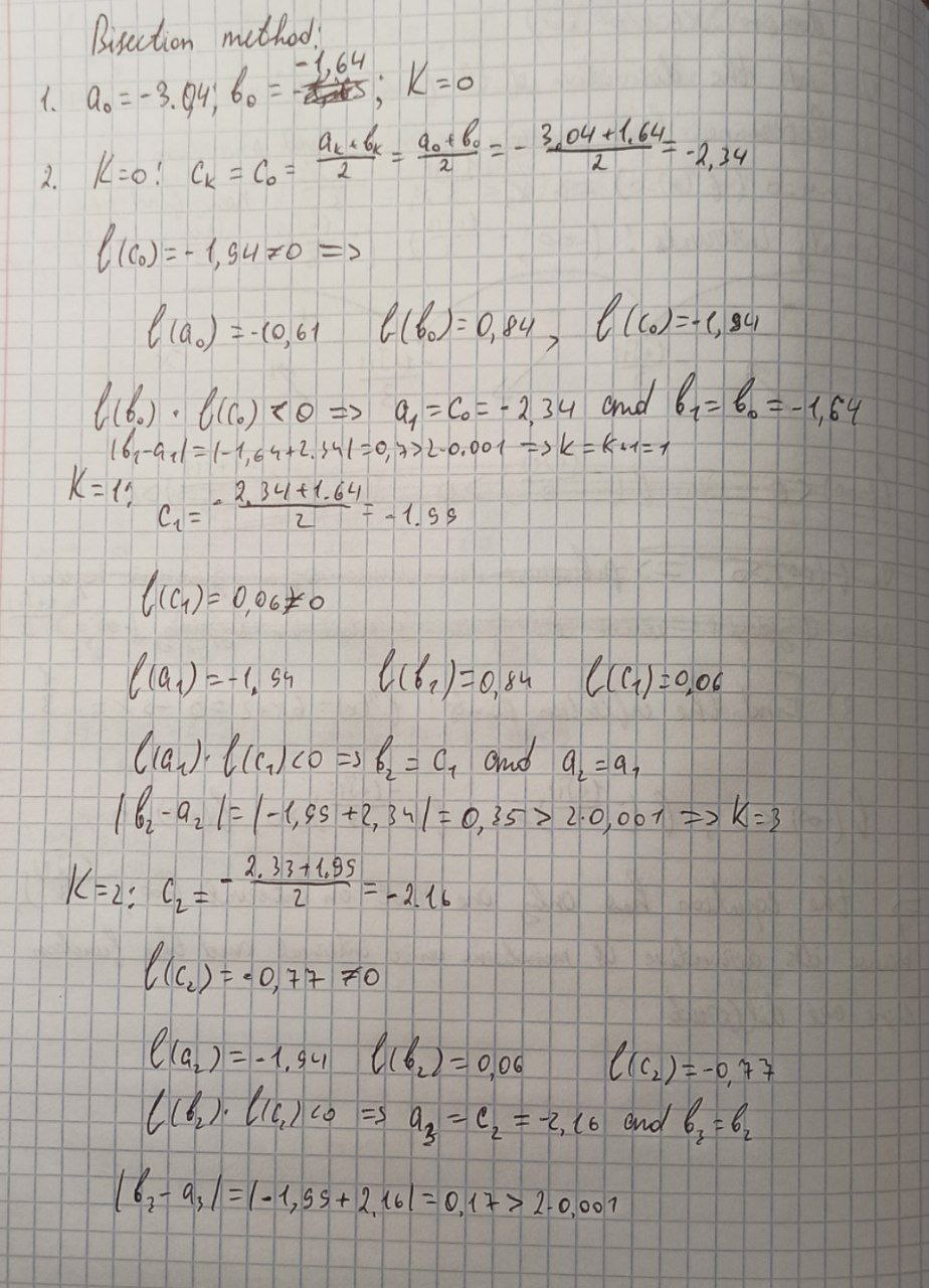
First method: Bisection method. The essence of the method is to find segments on which there is only one root, then consider each segment separately and carry out the following operations: 1. if the function in the middle of this segment takes the value zero, then the root is found, 2. If not, then the next taken segment is the one at the ends of which the function has different signs.
Manual solving:
Programming solving:
static void bisection_method() { std::vector<double> roots; std::vector<double> intervals = find_intervals();
int k = 0; for (size_t i = 0; i < intervals.size(); i += 2) { double ak = intervals[i]; double bk = intervals[i + 1]; double ck; if (!has_root_at_the_interval(ak, bk)) continue;
while (std::abs(ak - bk) >= 2 * epsilon) { ck = (ak + bk) / 2.;
if (f(ak) * f(ck) < 0) bk = ck;
else if (f(bk) * f(ck) < 0) ak = ck;
++k; } ck = (ak + bk) / 2.;
roots.emplace_back(ck); }
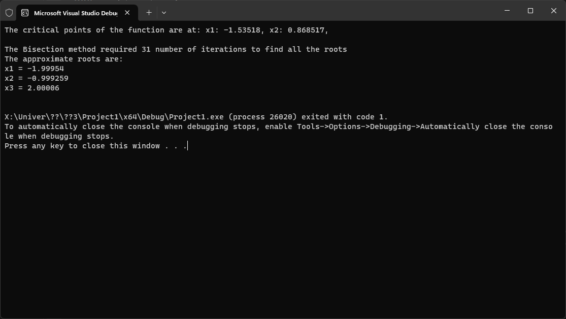
result_of_method("Bisection", roots, k); } |
The program’s output:
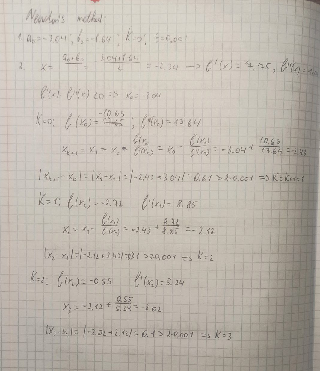
Second method: Newton’s method. The idea of this method is
that the arc of the graph on a very small segment [a, b] is replaced
by the tangent of the graph at this point, so the tangent to the
graph at this point is found, then its intersection with the abscissa
is found and then again find the tangent at this point and so on. The
process should be completed when the difference between the previous
value of point
 and
the current value
and
the current value
 is less than double the epsilon.
Manual solving:
Programming solving:
static void newtons_method() { std::vector<double> roots; std::vector<double> intervals = find_intervals();
int k = 0; for (size_t i = 0; i < intervals.size(); i += 2) {
if (!has_root_at_the_interval(intervals[i], intervals[i + 1])) continue;
double x0; double x = (intervals[i] + intervals[i + 1]) / 2;
if (value_of_first_derivative(x) * value_of_second_derivative(x) < 0) x = intervals[i]; else x = intervals[i + 1];
do { x0 = x; x = x - (f(x) / value_of_first_derivative(x));
++k; } while (std::abs(x0 - x) >= epsilon); roots.emplace_back(x); } result_of_method("Newton's", roots, k); } |
The program’s output:
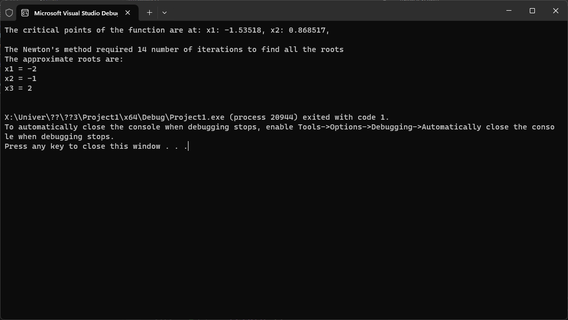
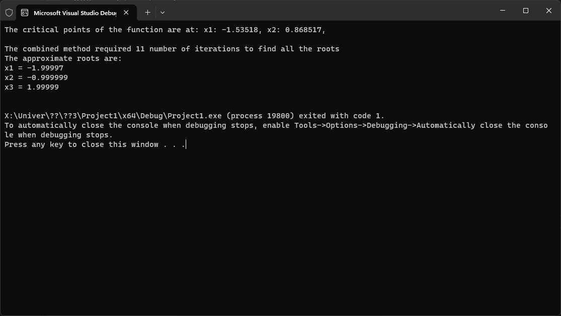
Third method: Combined method. The idea of the combined
method is that the chord method is used on one side of the
localization segment [a, b], and the tangent method is used on the
other side. In addition, the method also considers the placement of
the arc of the function graph on a given segment [a, b]; if both
derivatives have the same sign, then the chord method will determine
the value of the root with a shortage and the tangent method with a
surplus, and vice versa if the signs are different. The tangent
method was already explained so now about the chord: it’s similar
to bisection method but in there the values a and b are
divided by 2, here they are divided by the ration of numbers |f(a)|
and |f(b)|, i.e.
 .
.
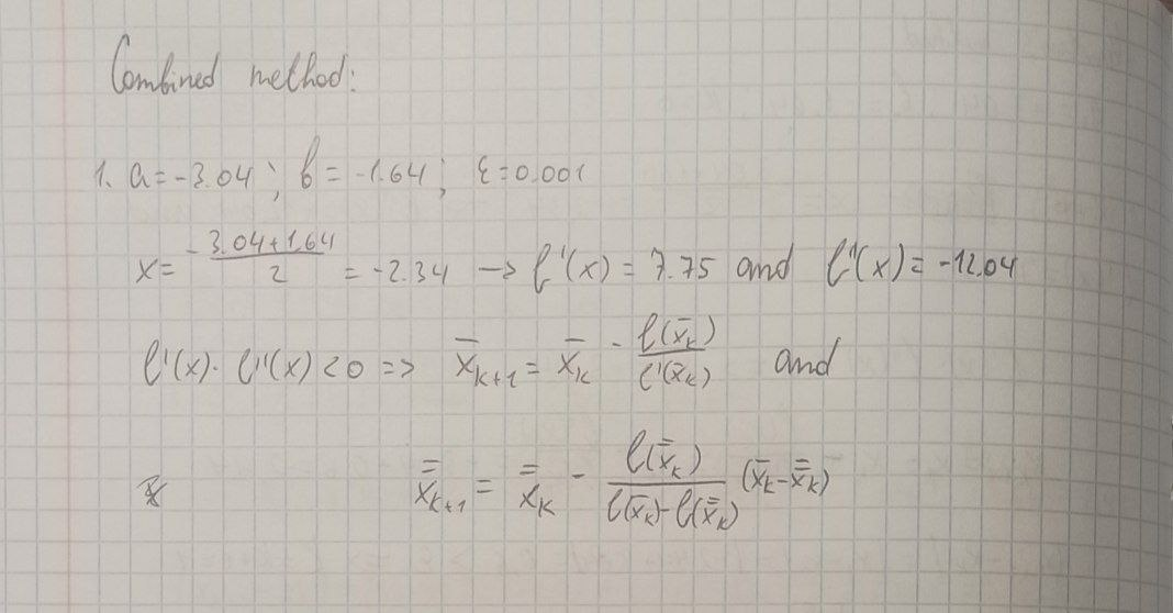
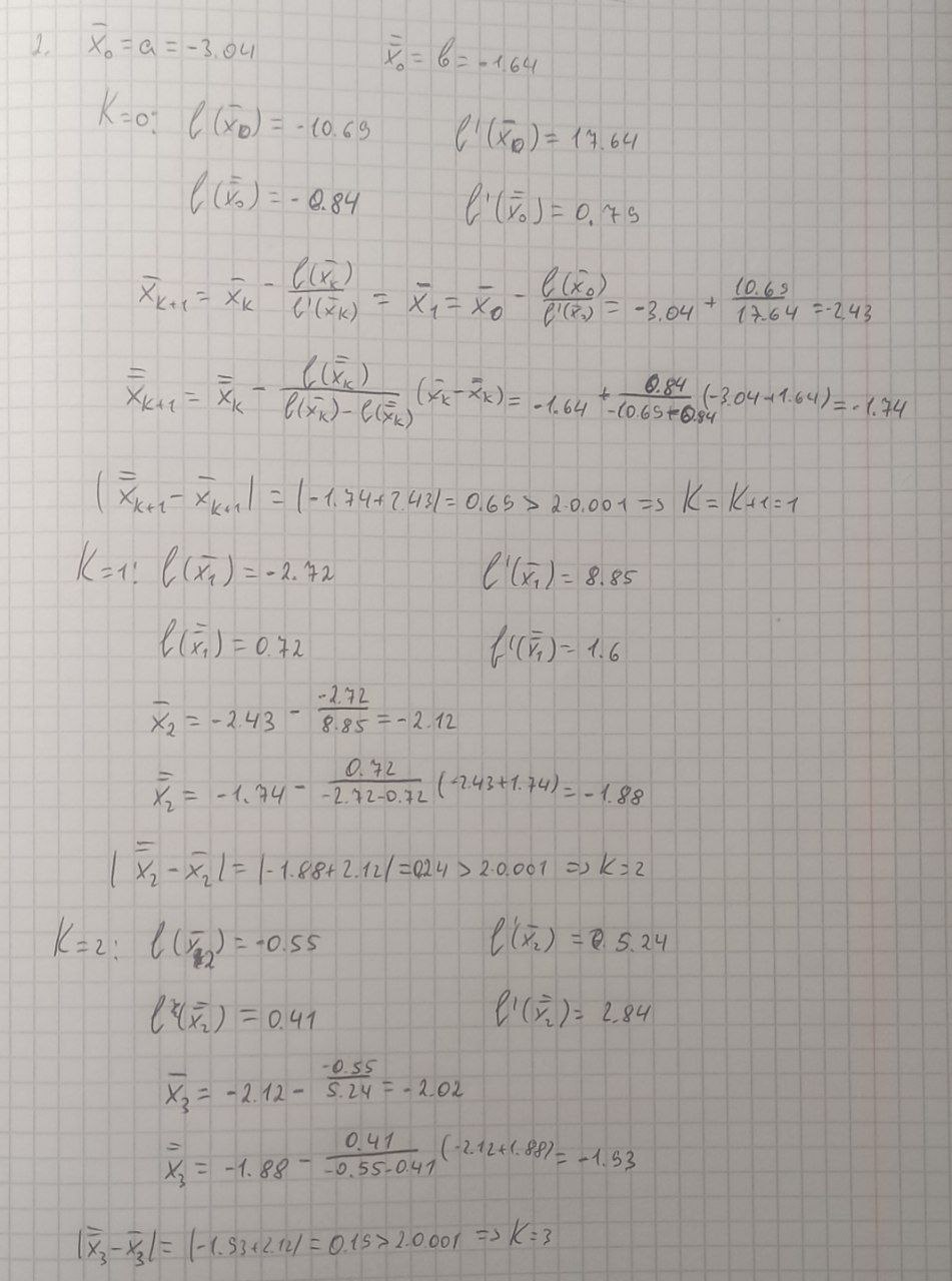
Manual solving:
Programming solving:
static void combined_method() { std::vector<double> roots; std::vector<double> intervals = find_intervals();
int k = 0; for (size_t i = 0; i < intervals.size(); i += 2) { //actually this step is uncessary because in 'find_intervals' we actually perform this check if (!has_root_at_the_interval(intervals[i], intervals[i + 1])) continue;
double a_k = (intervals[i] + intervals[i + 1]) / 2; double b_k;
if (value_of_first_derivative(a_k) * value_of_second_derivative(a_k) < 0) { a_k = intervals[i]; b_k = intervals[i + 1]; } else { b_k = intervals[i]; a_k = intervals[i + 1]; }
while (std::abs(a_k - b_k) > 2 * epsilon) { b_k = b_k - ( f(b_k) * (a_k - b_k) ) / ( f(a_k) - f(b_k) ); a_k = a_k - (f(a_k) / value_of_first_derivative(a_k));
++k; } double root = (a_k + b_k) / 2;
roots.emplace_back(root); } result_of_method("combined", roots, k); } |
The program’s output: