диафрагмированные волноводные фильтры / 6b097e10-038a-43ca-8c39-fcbbf8f4ed4a

ARTIFICIAL NEURAL NETWORK APPROACH FOR MODELING THE MICROSTRIP BANDPASS FILTER

Dr K Sri Rama Krishna1, K Jagadeesh Babu2 ,J Lakshmi Narayana3, G V Subrahmanyam4

#1 Professor & Head of ECE, V.R. Siddhartha Engineering College, Vijayawada, A.P, India #2,3 Associate Professor in ECE, St.Ann’s College of Engineering and Technology, A.P, India #4 Research Scholar in ECE, Acharya Nagarjuna University, Guntur, A.P, India

ABSTRACT

Artificial neural networks recently gained attention as a fast and flexible vehicle to microwave modeling and design. The advantage of using ANN models for filter design is a large saving in required CPU time. In this paper, an end coupled microstrip band-pass filter is designed to operate in the frequency range of 4GHz to 6GHz and its S-parameter responses are developed using ANN. Here the filter characteristics are analyzed using different learning algorithms like back propagation (MLP3), Quasi-Newton (MLP), Sparse training, Huber- Quasi-Newton, adaptive back propagation, auto pilot (MLP3) and conjugate gradient, and the results are compared with the simulated results in terms of correlation coefficient and average error.

Key words: Microstrip band-pass filter, Modeling, Artificial Neural Networks, Training algorithms.

Corresponding Author: K Sri Rama Krishna

I. INTRODUCTION

Recently, the millimeter wave band-pass filter has been studied and exploited extensively as a key circuit block in home networks, telematics, intelligent transport systems, and satellite highspeed Internet. Microstrip filters for RF/microwave applications offers a unique and comprehensive treatment of RF/microwave filters based on the microstrip structure, providing a link to applications of computer-aided design tools and advanced materials.

Microstrip lines are one of the most popular types of planar transmission lines, primarily because they can be fabricated by photolithographic processes and are easily integrated with other passive and active microwave devices. Fabrication of multi-section band-pass filters is particularly easy in microstrip line form, for bandwidth less than about 20%. These band-pass filters can be designed with various coupling mechanisms like edge coupling, parallel coupling and capacitive coupled resonators [1]. The designed filters can be operated in the S-Band frequency range yielding good results [2]. A microstrip band-pass filter can be designed and analyzed using different microwave CAD tools, however taking more simulation times. An EM based ANN model of the band-pass filter can give better and accurate results in shorter CPU times [3].

Recently a computer-aided-design (CAD) approach based on neural networks has been introduced for microwave modeling and design [4]–[6]. Neural networks are trained from

Page 162

measured/simulated microwave data and the resulting neural models are used during microwave design [7]. Neural modeling techniques have been applied to a wide variety of microwave problems, e.g., coplanar waveguide (CPW) components [7], transistors [8], transmission lines [9], bends [10], filters [11], and amplifiers [12]. Significant speed-up of CAD by using neural models in place of CPU intensive electromagnetic (EM)/physics models resulted in a drive to develop advanced neural modeling techniques [13]–[15].

The artificial neural network is considered as a grossly simplified model of the human brain. It is a computing system made up of a number of information processing units or artificial neurons highly interconnected through a set of links represented by synaptic weights, which are adjusted during a training process. Neural networks are widely applied to a variety of practical problems such as signal processing, speech processing, and control systems analysis and optimization of microwave circuits, telecommunications system design, intermodulation and power analysis and more.

Recently, artificial neural networks have become a popular tool in learning nonlinear maps from discrete data, due to their ability to learn from data, to generalize patterns in data, and to approximate any degree of non-linearity. Neural model development involves several subtasks like data generation, neural-network selection, training, and validation. Generally, these subtasks are manually carried out in a sequential manner independent of one another.

This paper presents simple and accurate analysis models based on ANNs in order to accurately compute the S-parameters of an end coupled band-pass filter for the required design specifications. ANN is a very powerful approach for building complex and non-linear relationship between a set of input and output data. ANNs have more general functional forms and are usually better than the classical techniques; also, they provide simplicity in real-time operation. One of the most powerful uses of ANNs is function approximation (curve fitting). A main characteristic of this solution is that a function (f) to be approximated is given not explicitly, but implicitly through a set of input-output pairs called training data sets.

II. ANN FOR ELECTROMAGNETIC APPLICATIONS

For a variety of problems, the neural network could substitute the EM analysis based on a software simulator tool once the learning process has been performed. To this end, some techniques have been defined in order to obtain the neural network that is capable of performing the required task by using the results obtained by EM simulations or the existing knowledge. In the field of microwave filters or more specifically in the field of microstrip filtering devices, the problem to be solved is that of the synthesis. In this case, the ANN must not only provide an alternative to the EM analysis tool, but it should also perform an analytical inversion. In other words, if the microwave filter produces as output the scattering parameters matrix S = ψ(p) where p is the array of the electromagnetic and geometrical parameters characterizing the filtering unit, the neural network must be able to determine p= ψ -1(s). Although inverse modeling is a tough problem, selectively choosing simulations (training data) helps.

Hence, the ANN has to be of the supervised type and the learning dataset considers the results given by the software simulator or the parameters obtained by laboratory test measurements as the ANN inputs and the geometrical and electromagnetic parameters of the filtering unit as outputs. This procedure is shown in Fig.1.

Page 163

Fig.1 Flow chart of the procedure for the determination of a feed forward ANN model

This approach allows us to obtain a suitable learning data set in a simple and straight forward way. In fact, the dependence of the S matrix with respect to the geometrical and EM parameters can be easily obtained from the software simulator data by modifying the parameter values. In this phase, it is easy to select the most learning patterns, avoiding at the same time to repeat the same patterns or those with a poor content of information. In other words, the learning data set determination phase, is in general a difficult and fundamental step in the correct development of the ANN model. Furthermore, the number of independent parameters that affect the learning pattern data set is already known; hence, the number of ANN outputs can be immediately developed.

III. FREQUENCY-DOMAIN NEURAL MODEL

Frequency-domain neural models are important for CAD such as nonlinear optimization of microstrip filters in the frequency domain. A frequency-domain neural model represents S parameters of a filter with the speed of empirical models, but with accuracy comparable to detailed EM models. In this section, formulation for training frequency domain neural models from frequency domain EM data is presented. Let x represent an Nx-vector containing the external inputs (stimuli) and y represent an Ny-vector containing the outputs (responses) of a filter. For example, x could contain parameters such as frequency of operation ‘f’ and y represents output parameters such as S-parameters or Y-parameters. Let f represent a detailed EM relation between x and y i.e.,

to be modeled by a neural network. Information of f can be typically accessed through detailed EM simulation software

Page 164

also referred to as an EM simulator. We introduce a terminology for simulator “g” and refer to it as a “data generator.” For a given input x , data generator can be used to compute the outputs d. Data generation involves repetitive use of g to obtain sample pairs (xk ,dk) where k is the sample index. These sample pairs are divided into training and test sets. We define Tr and Ts as index sets of training and test data, respectively. The purpose of neural-network modeling is to develop a fast neural model.

Y=fANN(x,w) (8)

that accurately represents g. Here fANN is a neural network trained to learn g from training data (xk , dk ), k Є Tr , Y is an Ny-vector of neural model responses, and w is an ANN weight vector.

The MLP network is the most commonly used neural network. For the purpose of ANN training, an error function is defined as

(9)

Here, yjk is the jth element of the neural-network output and djk is the jth element of corresponding data output .The objective of neural-network training is to adjust w such that E(w) is minimized. Following (10), we can also define a test error and use test data (xk , dk ) and k Є Ts to independently assess the quality of the trained neural model. The trained neural model fANN can be used in place of a CPU-intensive EM simulator to provide fast EM information needed during frequency-domain simulation and optimization.

Typically feed-forward layered networks consists of a set of source nodes which constitute the input layer, one or more hidden layers of computation nodes and an output layer of computation nodes. In Fig.2, the structure of a three layer neural network is represented. Each processing node (neuron) performs a weighted sum of the signal components at its input; this sum is thus fed into a block performing a differentiable nonlinear processing, usually a sigmoidal logistic function of the type,

f(v)=1/1+exp(-v) (10)

The input signal propagates through the network in a forward direction, on a layer-by-layer basis. These networks are usually referred to as multilayer perceptrons (MLPs). The processing task to be performed is described by a set of input-output data (the training set): the network specializes to solve this task by modifying its parameters (weights) by means of an iterative optimization procedure (the learning procedure). The error backpropagation is a widely popular learning technique that provides an efficient and algorithms stable way to correct the network weights.

Page 165

Fig.2. A three-layer neural network

IV. ANALYSIS OF MICROSTRIP BAND-PASS FILTER USING ANN

ANN models are a kind of black box models, whose accuracy depends on the data presented to it during training. A good collection of the training data, i.e., data which is well distributed, sufficient, and accurately simulated, is the basic requirement to obtain an accurate model. For microwave applications, there are two types of data generators, namely measurement and simulation. The selection of a data generator depends on the application and the availability of the data generator.

In this paper, the band-pass filter is designed using microstrip lines with length 11mm and width 0.645mm taken on a substrate with thickness 0.197mm and εr equals to 2.20. The coupling gaps for the microstrip lines are taken as 0.645mm and 0.780mm.These values are calculated using the formulas mentioned in (1) to (7) to operate in the frequency range of 4GHz to 6GHz. Once the filter is designed its response is evaluated in terms of its S-parameters (magnitude and angles of S11 and S12) for the mentioned frequency range using EM-simulator (Ansoft Designer). These obtained responses can be taken as the train data for the neural network. Here a training set of 400 samples is built using the simulator.

In the present discussion, the neural network-learning phase has to be carried out in order to generalize the information inside the training set, instead of providing a classification. The number of neurons and the other neural network parameters have been determined by heuristic considerations, taking into account the needs described above. The learning phase is carried out until the root mean square error computed on the outputs is close to 1%. A not so small root mean square error, yield a neural network, which has generalized the information, contained in the training set.

Once this value for the root mean square error is reached, the ANN has to synthesize the filters contained in the test set, which are not included in the training set. If the root mean square error remains of the same order of magnitude and the EM analysis of the filters shows that they satisfy the requirements, the learning process is stopped; otherwise, the ANN structure is changed and the learning procedure continues. If this process is reiterated many times, the test set becomes a part of the training set, but this event has never occurred and the learning phase convergence is quite fast.

In this paper, the neural models are trained with different learning algorithms like Back propagation (MLP3), Sparse Training, Conjugate Gradient, Adaptive Back Propagation, QuasiNewton (MLP), Quasi-Newton, Huber-Quasi-Newton, Auto Pilot (MLP3), to obtain better performance and faster convergence with a simpler structure. For the validation of the neural

Page 166

models proposed in this paper, the neural analysis results are compared with the results of the simulator.

V. RESULTS

ANNs have been successfully used to obtain the S-parameters of the end coupled microstrip band-pass filter in the frequency range of 4GHz to 6GHz. To evaluate the validity of neural networks in designing the microstrip filters, the various S-parameters like magnitude of S11, magnitude of S12, angle of S11 and angle of S12 are taken individually from the EM-simulator and these values are used to train the different ANN training algorithms like Back propagation (MLP3), Sparse Training, Conjugate Gradient, Adaptive Back Propagation, Quasi-Newton (MLP), Quasi-Newton, Huber-Quasi-Newton, Auto Pilot (MLP3) etc. Once the training is completed, next the test data (different from training data), which is generated in the same way from the simulator is processed by using the above mentioned algorithms and the results are compared in terms of training error, testing error and correlation coefficient.

TABLE I shows the training error, avg. testing error and correlation coefficients obtained by training the samples of S-parameters in the frequency range 4 GHz to 6 GHz with different learning algorithms. Here the correlation coefficient shows the amount of similarity between EM simulated results and ANN computed results. These values are compared with the values obtained from different learning algorithms mentioned above, and from the data shown in the tables, it is clear that Auto Pilot (MLP3) algorithm yields the better results compared to others.

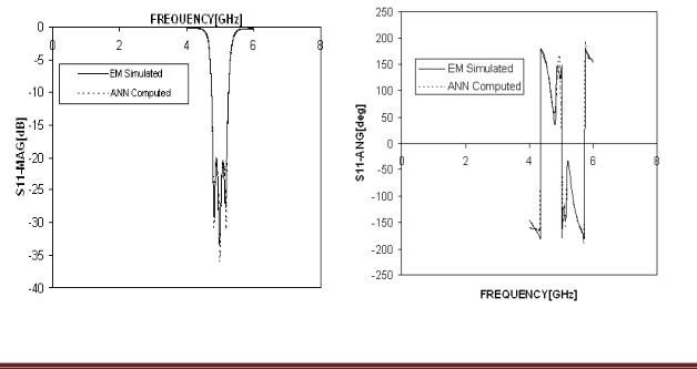
Using this algorithm the correlation coefficients of S11-Magnitude, S11-Angle, S12-Magnitude and S12-Angle are 0.9998, 0.9619, 0.9999 and 0.9988 respectively, which shows the similarity between EM simulated results and ANN computed results. From the table it is also evident that Auto Pilot (MLP3) algorithm gives the minimum training and testing errors. Comparisons between the EM simulated and ANN computed values for various S-parameters are shown in Fig. 3 and Fig.4. Because of the higher correlation between the values, the curves of EM simulated and ANN computed are almost all merged as shown in the mentioned figures.

(a) (b)

Fig. 3 Comparison between EM simulated and ANN Results (a) S11 Magnitude (b) S11 Phase

Page 167

Fig. 4 Comparison between EM simulated and ANN Results (a) S21 Magnitude (b) S21 Phase

TABLE I

TRAINING, TESTING ERRORS AND CORRELATION COEFFICIENTS

OF S11 AND S21 PARAMETER USING ANN MODEL

Page 168

VI. CONCLUSION

We presented the accurate and simple neural models to compute the S-parameters of an end coupled microstrip band-pass filter for the required design specifications. These models have been developed by training the neural network with the EM simulated results in the required frequency range (4 GHz to 6 GHz). Neural models were trained by using eight different learning algorithms to obtain better performance and faster convergence with a simpler structure. It was shown that the results of the neural models trained by the Auto Pilot (MLP3) algorithm are better than those of the neural models trained by other algorithms.

REFERENCES

[1]S. Prabhu and J. S. Mandeep, “Microstrip Band-pass Filter at S Band using Capacitive

Coupled Resonator”, Progress In Electromagnetics Research, PIER 76, 223–228, 2007

[2]Mohd Fadzil Ain, Mandeep Singh Jit Singh, Prabhu, Syed Idris Syed Hassan, “Design of a Symmetrical Microstrip Band-pass Filter for S-Band Frequency Range”, American Journal of Applied Sciences 4 (7): 426-429, 2007

[3]L. Jin, C. -L. Ruan, and L.-Y. Chun, Design E-Plane Band-pass Filter based on EM-ANN

Model”, J. of Electromagn. Waves and Appl., Vol. 20, No. 8, 1061–1069, 2006

[4]V. K. Devabhaktuni, M. C. E. Yagoub, Y. Fang, J. Xu, and Q. J. Zhang, “Neural networks for microwave modeling: Model development issues and nonlinear modeling techniques,” Int. J. RF Microwave CAE, vol. 11, pp. 4–21, 2001.

[5]Q. J. Zhang and K. C. Gupta, Neural Networks for RF and Microwave Design. Norwood, MA: Artech House, 2000.

Page 169