8 - Chapman MATLAB Programming for Engineers

average magnitude = 15 (|0.25| + |0.82| + | − 0.11| + | − 0.02| + |0.15|) = 0.270

average power = 15 0.252 + 0.822 + (−0.11)2 + (−0.02)2 + 0.152 = 0.154

number of zero crossings = 2

The Matlab commands to compute and write a wave file test.wav containing the test sequence:

>>x = [0.25 0.82 -0.11 -0.02 0.15]

>>wavwrite(x,’test.wav’)

Executing the script digit.m on the test data:

>> digit

Enter name of wave file as a string: ’test.wav’

Digit Statistics

samples: 5

sampling frequency: 8000.0 bits per sample: 16

mean: 0.2180

standard deviation: 0.3648 average magnitude: 0.2700 average power: 0.1540

zero crossings: 2

Observe that the results from the script agree with the hand-calculated values, giving us some confidence in the script.

Executing the script on a wave file zero.wav created using the “Sound Recorder” program on a PC to record the spoken word “zero” as a wave file:

>> digit

Enter name of wave file as a string: ’zero.wav’

Digit Statistics

samples: 13493

sampling frequency: 11025.0

177

bits per sample: 8 mean: -0.0155

standard deviation: 0.1000 average magnitude: 0.0690 average power: 0.0102

zero crossings: 271

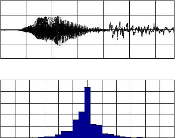
The resulting plots are shown in Figure 8.4.

Data sequence of spoken digit

Histogram of data sequence

5000

Figure 8.4: Data sequence and histogram for the spoken word ‘zero’

Observe that the characteristics of the change with time (index), as di erent sounds are being made to produce the word. An e ective word recognition algorithm must capture this change in sounds, but the design of such an algorithm is beyond the material covered in this course. Note that the histogram has the appearance of a Gaussian or bell-shaped curve, with a mean near zero and a standard deviation of about 0.35, while the data sequence looks much di erent than the Gaussian random data sequence shown in Figure 7.1.

You can experiment with the PC Sound Recorder program to record wave files for other spoken digits and then process them with digit. In recording these files, you will need to make sure that the number of data samples in the recorded file is less than 16,384 if you are using the Student Version of Matlab. This requires using the “Telephone Quality” recording option and you may need to delete the silent sections at the beginning and end of the record.

You can also create wave files using Matlab and then listen to the signals in these files using PC Sound Recorder. For example, to compute and write a wave file containing 16000 samples in 2 seconds of an 800Hz sinusoid:

>> t = linspace(0,2,16000);

178

>>y = cos(2*pi*800*t);

>>wavwrite(y,’cosine.wav’)

179

Section 9

Vectors, Matrices and Linear Algebra

A matrix is a two-dimensional array, as introduced in Section 7.2, where matrix addressing and methods of array creation were described. In Section 7.3, scalar-array mathematics and element-by- element array mathematics were described. In this chapter, we present a set of matrix operations and functions that apply to the matrix as a unit, as opposed to individual elements in the matrix.

Review of Matrix DeÞnitions

1. Scalar: A matrix with one row and one column.

A = [3.5]

2. Vector: A matrix with one row (a row vector) or one column, ( a column vector).

3. Matrix: An example of a matrix with four rows and three columns:

00 −2

The elements in a matrix are denoted by cij, where i is the row index and j is the column index. For example c43 refers to the element in row 4 and column 3, and thus, c43 = −2 in the example above. If needed to avoid misinterpretation, the indexes can be separated by a comma, as in ci,j and c4,3. In Matlab, subscripts are indicated by parentheses, as in C(4,3).

180

9.1Vectors

We usually think of vectors as column vectors, written as

To indicate that x is a vector of n real numbers, we write

x Rn

Geometrically, Rn is n-dimensional space, and the notation x Rn means that x is a point in that space, specified by the n coordinates x1, x2, . . . xn. Figure 9.1 shows a vector in R3, drawn as an arrow from the origin to the point x.

Figure 9.1: A vector in R3

Vector Addition

Vectors with the same number of elements can be added and subtracted in a very natural way:

181

Inner or Dot Product

The inner product (x, y), also referred to as the dot product x · y, is a scalar sum of products

(x, y) = x · y = x1y1 + x2y2 + x3y3 + · · · + xnyn

For example, for

4−2

the inner product is

(x, y) = 4 · (−2) + (−1) · 5 + 3 · 2 = −7

Properties:

1.(x, y) = (y, x)

2.(ax, y) = a(x, y) = (x, ay)

3.(x, y + z) = (x, y) + (x, z)

In Matlab, the inner product is computed with the dot function:

dot(x,y) Returns the scalar dot product of the vectors x and y, which must be of the same length.

dot(A,B) Returns a row vector of the dot products for the corresponding columns of matrices A and B.

Example:

>>x = [4 -1 3]’ x =

4 -1 3

>>y = [-2 5 2]’ y =

-2 5 2

>>d = dot(x,y) d =

-7

182

Euclidean Norm

The length of a vector is called the norm of the vector. From Euclidean geometry, the distance between two points is the square root of the sum of the squares of the distances in each dimension. Thus, the notation and definition of the Euclidean norm is

||x|| = x21 + x22 + · · · + x2n

Note that the norm can be defined in terms of the inner product:

||x|| = (x, x)

For example, the norm of x above is

||x|| = 42 + (−1)2 + 32 = 5.1

In Matlab, norm(x) returns the Euclidean norm of row vector or column vector x.

For example, for x and y as defined above:

>>nx = norm(x) nx =

5.0990

>>ny = norm(y) ny =

5.7446

Triangle Inequality

This inequality, also called the Cauchy-Bernoulli-Schwarz (CBS) inequality, states that the absolute value of the inner product of vectors x and y is less than or equal to the norm of x times the norm of y, with equality if and only if y = αx

|(x, y)| ≤ ||x|| ||y||

Confirming this using the examples above:

>>abs(dot(x,y)) ans =

7

>>norm(x)*norm(y) ans =

29.2916

183

To confirm the equality condition, define z = 5x

>>z = 5*x

z =

20 -5 15

>>abs(dot(x,z)) ans =

130

>>norm(x)*norm(z) ans =

130

Unit Vectors

The unit vector ux is a vector of length one pointing in the same direction as x

1 ux = ||x||x

>>ux = x/norm(x) ux =

0.7845 -0.1961 0.5883

>>norm(ux)

ans =

1

Angle Between Vectors

The angle θ between two vectors x and y is

(x, y) cos θ = ||x|| ||y||

>>theta = acos(dot(x,y)/(norm(x)*norm(y))) theta =

1.8121

>>thetad = (180/pi)*theta

thetad = 103.8261

184

Orthogonality

When the angle between two vectors is π/2 (90◦), the vectors are said to be orthogonal. From the equation for the angle between two vectors

(x, y) = 0 x and y are orthogonal

Projection

The projection of vector x onto y is found by dropping a perpendicular from the head of x onto the line representing y, as shown in Figure 9.2. The point where the perpendicular intersects y (or an extension of y) is the projection of x onto y, or the component of x in the direction of y. Denoting the projection vector by z

Figure 9.2: Projection of x onto y

>> z = (dot(x,y)/norm(y)^2)*y z =

0.4242 -1.0606 -0.4242

Example 9.1 Ship course

Figure 9.1 shows a ship sailing on bearing 315◦ (NW) with a speed of 20 knots. The local current due to the tide is 2 knots in the direction 67.5◦ (ENE). The ship also drifts at 0.5 knots under wind in the direction 180◦.

The following script is written to do the following:

•Represent the ship velocity as a vector S, the current velocity as a vector C, and the wind-drift velocity as a vector W. Calculate the true-velocity vector T (velocity over the ocean bottom). North represents the first component and East the second component of the vectors.

185

Figure 9.3: Ship course components

•Calculate the true ship speed, that is, the ship speed over the ocean bottom.

•Calculate the true ship course, that is, the direction of sailing over the ocean bottom, measured in degrees clockwise from north.

The function atan2 was used to compute the course heading, as it provides a four-quadrant result. However, it produces results in the range −π to π, which have to be converted to degrees in the range 0 to 360.

The displayed results:

Ship velocity vector:

S =

14.1421 -14.1421 Current velocity vector:

186