C H A P T E R T W E N T Y - F O U R

HOW DO YOU estimate the present value of a company’s bonds? The answer is simple: You take the cash flows and discount them at the opportunity cost of capital. Therefore, if a bond produces cash flows of C dollars per year for N years and is then repaid at its face value ($1,000), the present value is
PV |
|
C |
|
|
C |
… |
C |
|
|
|
$1,000 |
|
r |
|
1 1 r 2 2 |
1 1 r |
2 N |
|
1 r |
2 N |
1 |
1 |
|
|
1 |
|
|
|
|
2 |
|
N |
|
|
|
N |
|
where r1, r2, . . . , rN are the appropriate discount rates for the cash flows to be received by the bond owners in periods 1, 2, . . . , N.
That is correct as far as it goes but it does not tell us anything about what determines the discount rates. For example,
•In 1945 U.S. Treasury bills offered a return of .4 percent: At their 1981 peak they offered a return of over 17 percent. Why does the same security offer radically different yields at different times?
•In mid-2001 the U.S. Treasury could borrow for one year at an interest rate of 3.4 percent, but it had to pay nearly 6 percent for a 30-year loan. Why do bonds maturing at different dates offer different rates of interest? In other words, why is there a term structure of interest rates?
•In mid-2001 the United States government could issue long-term bonds at a rate of nearly 6 percent. But even the most blue-chip corporate issuers had to pay at least 50 basis points (.5 percent) more on their long-term borrowing. What explains the premium that firms have
to pay?
These questions lead to deep issues that will keep economists simmering for years. But we can give general answers and at the same time present some fundamental ideas.
Why should the financial manager care about these ideas? Who needs to know how bonds are priced as long as the bond market is active and efficient? Efficient markets protect the ignorant trader. If it is necessary to know whether the price is right for a proposed bond issue, you can check the prices of similar bonds. There is no need to worry about the historical behavior of interest rates, about the term structure, or about the other issues discussed in this chapter.
We do not believe that ignorance is desirable even when it is harmless. At least you ought to be able to read the bond tables in The Wall Street Journal and talk to investment bankers about the prices of recently issued bonds. More important, you will encounter many problems of bond pricing where there are no similar instruments already traded. How do you evaluate a private placement with a custom-tailored repayment schedule? How about financial leases? In Chapter 26 we will see that they are essentially debt contracts, but often extremely complicated ones, for which traded bonds are not close substitutes. Many companies, notably banks and insurance firms, are exposed to the risk of interest rate fluctuations. To control their exposure, these companies need to understand how interest rates change.1 You will find that the terms, concepts, and facts presented in this chapter are essential to the analysis of these and other practical problems.
We start the chapter with our first question: Why does the general level of interest rates change over time? Next we turn to the relationship between shortand long-term interest rates. We consider three issues:
•Each period’s cash flow on a bond potentially needs to be discounted at a different interest rate, but bond investors often calculate the yield to maturity as a summary measure of the interest rate on the bond. We first explain how these measures are related.
continued
1We discuss in Chapter 27 how firms protect themselves against interest rate risk.
668PART VII Debt Financing
•Second, we show why a change in interest rates has a greater impact on the price of long-term loans than on short-term loans.
•Finally, we look at some theories that explain why shortand long-term interest rates differ. To close the chapter we shift the focus to corporate bonds and examine the risk of default and its effect on bond prices.
24.1 REAL AND NOMINAL RATES OF INTEREST
Indexed Bonds and the Real Rate of Interest
In Chapter 3 we drew the distinction between the real and nominal rate of interest. Most bonds promise a fixed nominal rate of interest. The real interest rate that you receive depends on the inflation rate. For example, if a one-year bond promises you a return of 10 percent and the expected inflation rate is 4 percent, the expected real return on your bond is 1.10/1.04 1 .058, or 5.8 percent. Since future inflation rates are uncertain, the real return on a bond is also uncertain. For example, if inflation turns out to be higher than the expected 4 percent, the real return will be lower than 5.8 percent.
You can nail down a real return; you do so by buying an indexed bond whose payments are linked to inflation. Indexed bonds have been around in many countries for decades, but they were almost unknown in the United States until 1997 when the U.S. Treasury began to issue inflation-indexed bonds known as TIPs (Treasury Inflation-Protected Securities).2
The real cash flows on TIPs are fixed, but the nominal cash flows (interest and principal) are increased as the Consumer Price Index increases. For example, suppose that the U.S. Treasury issues 3 percent 20-year TIPs at a price of 100. If during the first year the Consumer Price Index rises by (say) 10 percent, then the coupon payment on the bond would be increased by 10 percent to 1 1.1 3 2 3.3 percent. And the final payment of principal would also be increased in the same proportion to 1 1.1 100 2 110 percent. Thus, an investor who buys the bond at the issue price and holds it to maturity can be assured of a real yield of 3 percent.
As we write this in the summer of 2001, long-term TIPs offer a yield of 3.46 percent. This yield is a real yield: It measures how much extra goods your investment would allow you to buy. The 3.46 percent yield on TIPs was about 2.3 percent less than on nominal Treasury bonds. If the annual inflation rate proves to be higher than 2.3 percent, you will earn a higher return by holding long-term TIPs; if the inflation rate is lower than 2.3 percent, the reverse will be true.
What determines the real interest rate that investors demand? The classical economist’s answer to this question is summed up in the title of Irving Fisher’s great book: The Theory of Interest: As Determined by Impatience to Spend Income and Opportunity to Invest It.3 The real interest rate, according to Fisher, is the price which equates
2In 1988 Franklin Savings Association had issued a 20-year bond whose interest (but not principal) was tied to the rate of inflation. Since then a trickle of companies has also issued indexed bonds.
3August M. Kelley, New York, 1965; originally published in 1930.
CHAPTER 24 Valuing Debt |
669 |
|
14 |
|
|
|
|
|
|
|
|
|
|
|
|
|
|
|
|
|
|
12 |
|
|
|
|
|
|
|
|
|
|
|
|
|
|
|
|
|
Percent |
10 |
|
|
|
|
|
|
|
|
Yield on UK nominal bonds |
|
|
|
|
|
|
|
|
|
|
|
8 |
|
|
|
|
|
|
|
|
|
|
|
|
|
|
|
|
|
6 |
|
Real yield on UK indexed bonds |
|
|
|
|
|
|
|
|
|
4 |
|
|
|
|
|
|
|
|
|
|
|
|
|
|
|
|
|
|
2 |
|
|
|
|
|
|
|
|
|
|
|
|
|
|
|
|
|
|
0 |
|
|
|
|
|
|
|
|
|
|
|
|
|
|
|
|
|
|
Dec. 83 |
Dec. 84 |
Dec. 85 |
Dec. 86 |
Dec. 87 |
Dec. 88 |
Dec. 89 |
Dec. 90 |
Dec. 91 |
Dec. 92 |
Dec. 93 |
Dec. 94 |
Dec. 95 |
Dec. 96 |
Dec. 97 |
Dec. 98 |
Dec. 99 |
Dec. 00 |
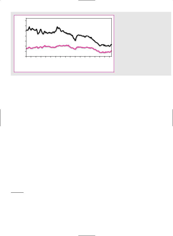
F I G U R E 2 4 . 1
The burgundy line shows the real yield on long-term indexed bonds issued by the UK government. The blue line shows the yield on UK government long-term nominal bonds. Notice that the real yield has been much more stable than the nominal yield.
the supply and demand for capital. The supply depends on people’s willingness to save.4 The demand depends on the opportunities for productive investment.
For example, suppose that investment opportunities generally improve. Firms have more good projects, so they are willing to invest more than previously at any interest rate. Therefore, the rate has to rise to induce individuals to save the additional amount that firms want to invest.5 Conversely, if investment opportunities deteriorate, there will be a fall in the real interest rate.
Fisher’s theory emphasizes that the required real rate of interest depends on real phenomena. A high aggregate willingness to save may be associated with high aggregate wealth (because wealthy people usually save more), an uneven distribution of wealth (an even distribution would mean fewer rich people, who do most of the saving), and a high proportion of middle-aged people (the young don’t need to save and the old don’t want to—“You can’t take it with you”). Correspondingly, a high propensity to invest may be associated with a high level of industrial activity or major technological advances.
Real interest rates do change but they do so gradually. We can see this by looking at the UK, where the government has issued indexed bonds since 1982. The colored line in Figure 24.1 shows that the (real) yield on these bonds has fluctuated within a relatively narrow range, while the yield on nominal government bonds has declined dramatically.
Inflation and Nominal Interest Rates
Now let us see what Irving Fisher had to say about inflation and interest rates. Suppose that consumers are equally happy with 100 apples today or 105 apples in a year’s time. In this case the real or “apple” interest rate is 5 percent. Suppose also
4Some of this saving is done indirectly. For example, if you hold 100 shares of GM stock, and GM retains earnings of $1 per share, GM is saving $100 on your behalf.
5We assume that investors save more as interest rates rise. It doesn’t have to be that way; here is an example of how a higher interest rate could mean less saving: Suppose that 20 years hence you will need $50,000 at current prices for your children’s college expenses. How much will you have to set aside today to cover this obligation? The answer is the present value of a real expenditure of $50,000 after 20 years, or 50,000/ 1 1 real interest rate 2 20. The higher the real interest rate, the lower the present value and the less you have to set aside.
670 |
PART VII Debt Financing |
that I know the price of apples will increase over the year by 10 percent. Then I will part with $100 today if I am repaid $115 at the end of the year. That $115 is needed to buy me 5 percent more apples than I can get for my $100 today. In other words, the nominal, or “money,” rate of interest must equal the required real, or “apple,” rate plus the prospective rate of inflation.6 A change of 1 percent in the expected inflation rate produces a change of 1 percent in the nominal interest rate. That is Fisher’s theory: A change in the expected inflation rate will cause the same change in the nominal interest rate; it has no effect on the required real interest rate.7
Nominal interest rates cannot be negative; if they were, everyone would prefer to hold cash, which pays zero interest.8 But what about real rates? For example, is it possible for the money rate of interest to be 5 percent and the expected rate of inflation to be 10 percent, thus giving a negative real interest rate? If this happens, you may be able to make money in the following way: You borrow $100 at an interest rate of 5 percent and you use the money to buy apples. You store the apples and sell them at the end of the year for $110, which leaves you enough to pay off your loan plus $5 for yourself.
Since easy ways to make money are rare, we can conclude that if it doesn’t cost anything to store goods, the money rate of interest can’t be less than the expected rise in prices. But many goods are even more expensive to store than apples, and others can’t be stored at all (you can’t store haircuts, for example). For these goods, the money interest rate can be less than the expected price rise.
How Well Does Fisher’s Theory Explain Interest Rates?
Not all economists would agree with Fisher that the real rate of interest is unaffected by the inflation rate. For example, if changes in prices are associated with changes in the level of industrial activity, then in inflationary conditions I might want more or less than 105 apples in a year’s time to compensate me for the loss of 100 today.
We wish we could show you the past behavior of interest rates and expected inflation. Instead we have done the next best thing and plotted in Figure 24.2 the return on U.S. Treasury bills against actual inflation. Notice that between 1926 and 1981 the return on Treasury bills was below the inflation rate about as often as it
6We oversimplify. If apples cost $1.00 apiece today and $1.10 next year, you need 1.10 105 $115.50 next year to buy 105 apples. The money rate of interest is 15.5 percent, not 15. Remember, the exact formula relating real and money rates is
1 rmoney 1 1 rreal 2 1 1 i 2
where i is the expected inflation rate. Thus
rmoney rreal i i1 rreal 2
In our example, the money rate should be
rmoney .05 .10 .101 .05 2 .155
When we said the money rate should be 15 percent, we ignored the cross-product term i 1 rreal 2 . This is a common rule of thumb because the cross-product term is usually small. But there are countries where
i is large (sometimes 100 percent or more). In such cases it pays to use the full formula.
7The apple example was taken from R. Roll, “Interest Rates on Monetary Assets and Commodity Price Index Changes,” Journal of Finance 27 (May 1972), pp. 251–278.
8There seems to be an exception to almost every statement. In late 1998 concern about the solvency of some Japanese banks led to a large volume of yen deposits with Western banks. Some of these banks charged their customers interest on these deposits; the nominal interest rate was negative.
CHAPTER 24 Valuing Debt |
671 |
|
20 |
|
|
|
|
|
|
|
|
|
|
|
|
|
|
|
15 |
Inflation |
|
|
|
Treasury bill return |
|
|
|
|
|
|
|
|
|
|
|
|
|
|
|
|
|
|
10 |
|
|
|
|
|
|
|
|
|
|
|
|
|
|
Percent |
5 |
|
|
|
|
|
|
|
|
|
|
|
|
|
|
0 |
|
|
|
|
|
|
|
|
|
|
|
|
|
|
|
|
|
|
|
|
|
|
|
|
|
|
|
|
|
|
-5 |
|
|
|
|
|
|
|
|
|
|
|
|
|
|
|
-10 |
|
|
|
|
|
|
|
|
|
|
|
|
|
|
|
-15 |
|
|
|
|
|
|
|
|
|
|
|
|
|
|
|
1926 |
1931 |
1936 |
1941 |
1946 |
1951 |
1956 |
1961 |
1966 |
1971 |
1976 |
1981 |
1986 |
1991 |
1996 |
|
|
|
|
|
|
|
|
Year |
|
|
|
|
|
|
F I G U R E 2 4 . 2
The return on U.S. Treasury bills and the rate of inflation, 1926–2000.
Source: Ibbotson Associates, Inc.,
Chicago, 2001.
was above. The average real interest rate during this period was a mere 0.1 percent. Since 1981 the return on bills has been significantly higher than the rate of inflation, so that investors have earned a positive real return on their savings.
Fisher’s theory states that changes in anticipated inflation produce corresponding changes in the rate of interest. But Figure 24.2 offers little evidence of this in the 1930s and 1940s. During this period, the return on Treasury bills scarcely changed even though the inflation rate fluctuated sharply. Either these changes in inflation were unanticipated or Fisher’s theory was wrong. Since the early 1950s, there appears to have been a closer relationship between interest rates and inflation in the United States.9 Thus, for today’s financial managers Fisher’s theory provides a useful rule of thumb. If the expected inflation rate changes, it is a good bet that there will be a corresponding change in the interest rate.
24.2 TERM STRUCTURE AND YIELDS TO MATURITY
We turn now to the relationship between shortand long-term rates of interest. Suppose that we have a simple loan that pays $1 at time 1. The present value of this loan is
PV 1 1 r1
Thus we discount the cash flow at r1, the rate appropriate for a one-period loan. This rate, which is fixed today, is often called today’s one-period spot rate.
If we have a loan that pays $1 at both time 1 and time 2, present value is
9This probably reflects government policy, which before 1951 stabilized nominal interest rates. The 1951 “accord” between the Treasury and the Federal Reserve System permitted more flexible nominal interest rates after 1951.
672 |
PART VII Debt Financing |
Thus the first period’s cash flow is discounted at today’s one-period spot rate and the second period’s flow is discounted at today’s two-period spot rate. The series of spot rates r1, r2, etc., is one way of expressing the term structure of interest rates.
Yield to Maturity
Rather than discounting each of the payments at a different rate of interest, we could find a single rate of discount that would produce the same present value. Such a rate is known as the yield to maturity, though it is in fact no more than our old acquaintance, the internal rate of return (IRR), masquerading under another name. If we call the yield to maturity y, we can write the present value of the two-year loan as
All you need to calculate y is the price of a bond, its annual payment, and its maturity. You can then rapidly work out the yield with the aid of a preprogrammed calculator.
The yield to maturity is unambiguous and easy to calculate. It is also the stock- in-trade of any bond dealer. By now, however, you should have learned to treat any internal rate of return with suspicion.10 The more closely we examine the yield to maturity, the less informative it is seen to be. Here is an example.
Example. It is 2003. You are contemplating an investment in U.S. Treasury bonds and come across the following quotations for two bonds:11
|
|
Yield to Maturity |
Bond |
Price |
(IRR) |
5s of ‘08 |
85.21% |
8.78% |
10s of ‘08 |
105.43 |
8.62 |
The phrase “5s of ‘08” refers to a bond maturing in 2008, paying annual interest of 5 percent of the bond’s face value. The interest payment is called the coupon payment. In continental Europe coupons are usually paid annually; in the United States they are usually paid every six months, so the 5s of ‘08 would pay 2.5 percent of face value every six months. To simplify the arithmetic, we will pretend throughout this chapter that all coupon payments are annual. When the bonds mature in 2008, bondholders receive the bond’s face value in addition to the final interest payment.
The price of each bond is quoted as a percent of face value. Therefore, if face value is $1,000, you would have to pay $852.11 to buy the bond and your yield would be 8.78 percent. Letting 2003 be t 0, 2004 be t 1, etc., we have the following discounted-cash-flow calculation:
|
|
|
|
Cash Flows |
|
|
|
|
|
|
|
|
|
|
|
Bond |
C0 |
C1 |
C2 |
C3 |
C4 |
C5 |
Yield |
5s of ‘08 |
852.11 |
50 |
50 |
50 |
50 |
1,050 |
8.78% |
10s of ‘08 |
1,054.29 |
100 |
100 |
100 |
100 |
1,100 |
8.62 |
|
|
|
|
|
|
|
|
10See Section 5.3.
11The quoted bond price is known as the flat (or clean) price. The price that the bond buyer pays (sometimes called the dirty price) is equal to the flat price plus the interest that the seller has already earned on the bond since the last interest payment date. You need to use the flat price to calculate yields to maturity.
CHAPTER 24 Valuing Debt |
673 |
|
|
|
|
|
Present Value Calculations |
|
|
|
|
|
|
|
|
|
|
|
|
|
|
|
|
|
Interest |
|
|
5s of ‘08 |
|
|
|
10s of ‘08 |
|
|
|
|
|
|
|
|
|
|
|
|
|
|
|
|
|
|
|
|
|
|
|
|
|
|
|
|
Period |
Rate |
|
|
Ct |
PV at rt |
|
|
Ct |
|
PV at rt |
t 1 |
r1 .05 |
$ |
50 |
$ 47.62 |
|
$ |
100 |
$ |
95.24 |
|
t 2 |
r2 .06 |
|
|
50 |
44.50 |
|
|
100 |
|
|
89.00 |
|
t 3 |
r3 .07 |
|
|
50 |
40.81 |
|
|
100 |
|
|
81.63 |
|
t 4 |
r4 .08 |
|
|
50 |
36.75 |
|
|
100 |
|
|
73.50 |
|
t 5 |
r5 .09 |
|
|
1,050 |
|
682.43 |
|
|
1,100 |
|
|
714.92 |
|
|
|
|
|
|
|
|
|
|
|
|
|
|
|
|
Totals |
|
|
|
|
$852.11 |
|
|
|
|
$1,054.29 |
|
|
|
|
|
|
|
|
|
|
|
|
|
|
|
|
T A B L E 2 4 . 1
Calculating present value of two bonds when long-term interest rates are higher than short-term rates.
Although the two bonds mature at the same date, they presumably were issued at different times—the 5s when interest rates were low and the 10s when interest rates were high.
Are the 5s of ‘08 a better buy? Is the market making a mistake by pricing these two issues at different yields? The only way you will know for sure is to calculate the bonds’ present values by using spot rates of interest: r1 for 2004, r2 for 2005, etc. This is done in Table 24.1.
The important assumption in Table 24.1 is that long-term interest rates are higher than short-term interest rates. We have assumed that the one-year interest rate is r1 .05, the two-year rate is r2 .06, and so on. When each year’s cash flow is discounted at the rate appropriate to that year, we see that each bond’s present value is exactly equal to the quoted price. Thus each bond is fairly priced.
Why do the 5s have a higher yield? Because for each dollar that you invest in the 5s you receive relatively little cash inflow in the first four years and a relatively high cash inflow in the final year. Therefore, although the two bonds have identical maturity dates, the 5s provide a greater proportion of their cash flows in 2008. In this sense the 5s are a longer-term investment than the 10s. Their higher yield to maturity just reflects the fact that long-term interest rates are higher than shortterm rates.
Notice why the yield to maturity can be misleading. When the yield is calculated, the same rate is used to discount all payments on the bond. But in our example bondholders actually demanded different rates of return (r1, r2, etc.) for cash flows that occurred at different times. Since the cash flows on the two bonds were not identical, the bonds had different yields to maturity. Therefore, the yield to maturity on the 5s of ‘08 offered only a rough guide to the appropriate yield on the 10s of ‘08.12
Measuring the Term Structure
Financial managers who just want a quick, summary measure of interest rates look in the financial press at the yields to maturity on government bonds. Thus managers will make broad generalizations such as “If we borrow money today, we will have to pay an interest rate of 8 percent.” But if you wish to understand why different
12For a good analysis of the relationship between the yield to maturity and spot interest rates, see S. M. Schaefer, “The Problem with Redemption Yields,” Financial Analysts Journal 33 (July–August 1977), pp. 59–67.
674 |
PART VII Debt Financing |
F I G U R E 2 4 . 3
Spot rates on U.S. Treasury strips, June 2001.
|
7 |
|
|
|
|
|
percent |
6 |
|
|
|
|
|
5 |
|
|
|
|
|
4 |
|
|
|
|
|
rate, |
|
|
|
|
|
3 |
|
|
|
|
|
Spot |
2 |
|
|
|
|
|
1 |
|
|
|
|
|
|
|
|
|
|
|
|
0 |
2006 |
2011 |
2016 |
2021 |
2026 |
|
2001 |
|
|
|
|
Year |
|
|
bonds sell at different prices, you must dig deeper and look at the separate interest rates for one-year cash flows, for two-year cash flows, and so on. In other words, you must look at the spot rates of interest.
To find the spot interest rate, you need the price of a bond that simply makes one future payment. Fortunately, such bonds do exist. They are known as stripped bonds or strips. Strips originated in 1982 when several investment bankers came up with a novel idea. They bought U.S. Treasury bonds and reissued their own separate mini-bonds, each of which made only one payment. The idea proved to be popular with investors, who welcomed the opportunity to buy the mini-bonds rather than the complete package. If you’ve got a smart idea, you can be sure that others will soon clamber onto your bandwagon. It was therefore not long before the Treasury issued its own mini-bonds.13 The prices of these bonds are shown each day in the daily press. For example, in the summer of 2001, a strip maturing in May 2021 cost $316.55 and 20 years later will give the investors a single payment of $1,000. Thus the 20-year spot rate was 1 1000/316.55 2 1/20 1 .0592, or 5.92 percent.14
In Figure 24.3 we have used the prices of strips with different maturities to plot the term structure of spot rates from 1 to 24 years. You can see that investors required an interest rate of 3.4 percent from a bond that made a payment only at the end of one year and a rate of 5.8 percent from a bond that paid off only in year 2025.
24.3 HOW INTEREST RATE CHANGES AFFECT BOND PRICES
Duration and Bond Volatility
In Chapter 7 we reviewed the historical performance of different security classes. We showed that since 1926 long-term government bonds have provided a higher average return than short-term bills, but have also been more variable. The stan-
13The Treasury continued to auction coupon bonds in the normal way, but investors could exchange them at the Federal Reserve Bank for stripped bonds.
14This is an annually compounded rate. The yields quoted by investment dealers are semiannually compounded rates.