CHAPTER 8 Risk and Return |
199 |
Average risk premium, 1931–1991, percent
30 |
|
|
|
|
|
|
|
|
|
|
25 |
|
|
|
|
|
|
|
|
Market |
|
20 |
|
|
|
|
|
|
|
|
line |
|
|
|
|
|
|
|
|
|
|
|
|
15 |
|
2 |
3 |
|
5 M |
6 |
8 |
9 |
Investor 10 |
|
Investor 1 |
|
|
7 |
|
|
|||||
10 |
|
|
|
4 |
Market |
|
|
|
||
|
|
|
|
|
|
|
||||
|
|
|
|
|
|
|
|
|||
5 |
|
|
|
|
portfolio |
|
|
|
||
|
|
|
|
|
|
|
|
|
|
Portfolio |
.2 |
.4 |
.6 |
.8 |
|
1.0 |
|
1.2 |
1.4 |
1.6 |
beta |
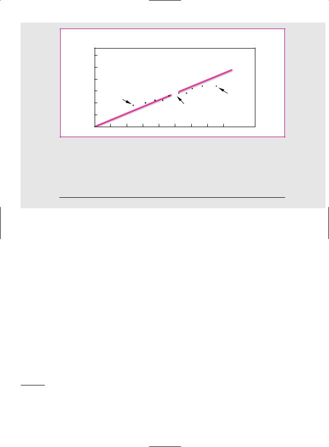
F I G U R E 8 . 9
The capital asset pricing model states that the expected risk premium from any investment should lie on the market line. The dots show the actual average risk premiums from portfolios with different betas. The high-beta portfolios generated higher average returns, just as predicted by the CAPM. But the high-beta portfolios plotted below the market line, and four of the five low-beta portfolios plotted above. A line fitted to the 10 portfolio returns would be “flatter” than the market line.
Source: F. Black, “Beta and Return,” Journal of Portfolio Management 20 (Fall 1993), pp. 8–18.
Tests of the Capital Asset Pricing Model
Imagine that in 1931 ten investors gathered together in a Wall Street bar to discuss their portfolios. Each agreed to follow a different investment strategy. Investor 1 opted to buy the 10 percent of New York Stock Exchange stocks with the lowest estimated betas; investor 2 chose the 10 percent with the next-lowest betas; and so on, up to investor 10, who agreed to buy the stocks with the highest betas. They also undertook that at the end of every year they would reestimate the betas of all NYSE stocks and reconstitute their portfolios.14 Finally, they promised that they would return 60 years later to compare results, and so they parted with much cordiality and good wishes.
In 1991 the same 10 investors, now much older and wealthier, met again in the same bar. Figure 8.9 shows how they had fared. Investor 1’s portfolio turned out to be much less risky than the market; its beta was only .49. However, investor 1 also realized the lowest return, 9 percent above the risk-free rate of interest. At the other extreme, the beta of investor 10’s portfolio was 1.52, about three times that of investor 1’s portfolio. But investor 10 was rewarded with the highest return, averaging 17 percent a year above the interest rate. So over this 60-year period returns did indeed increase with beta.
As you can see from Figure 8.9, the market portfolio over the same 60-year period provided an average return of 14 percent above the interest rate15 and (of
14Betas were estimated using returns over the previous 60 months.
15In Figure 8.9 the stocks in the “market portfolio” are weighted equally. Since the stocks of small firms have provided higher average returns than those of large firms, the risk premium on an equally weighted index is higher than on a value-weighted index. This is one reason for the difference between the 14 percent market risk premium in Figure 8.9 and the 9.1 percent premium reported in Table 7.1.
CHAPTER 8 Risk and Return |
201 |
Dollars |
|
(log scale) |
|
100 |
|
|
High minus low book-to-market |
10 |
|
|
Small minus large |
1 |
|
0.1 |
1932 1937 1942 1947 1952 1957 1962 1967 1972 1977 1982 1987 1992 1997 |
|
|
|
Year |
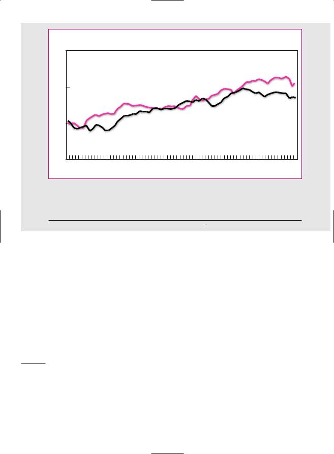
F I G U R E |
8 . 1 1 |
The burgundy line shows the cumulative difference between the returns on small-firm and large-firm stocks. The blue line shows the cumulative difference between the returns on high book-to-market- value stocks and low book-to-market-value stocks.
Source: www.mba.tuck.dartmouth.edu/pages/faculty/ken.french/data library.
erage investors have received the returns they expected. This noise may make it impossible to judge whether the model holds better in one period than another.16 Perhaps the best that we can do is to focus on the longest period for which there is reasonable data. This would take us back to Figure 8.9, which suggests that expected returns do indeed increase with beta, though less rapidly than the simple version of the CAPM predicts.17
The CAPM has also come under fire on a second front: Although return has not risen with beta in recent years, it has been related to other measures. For example, the burgundy line in Figure 8.11 shows the cumulative difference between the returns on small-firm stocks and large-firm stocks. If you had bought the shares with the smallest market capitalizations and sold those with the largest capitalizations, this is how your wealth would have changed. You can see that small-cap stocks did not always do well, but over the long haul their owners have made substantially
16A second problem with testing the model is that the market portfolio should contain all risky investments, including stocks, bonds, commodities, real estate—even human capital. Most market indexes contain only a sample of common stocks. See, for example, R. Roll, “A Critique of the Asset Pricing Theory’s Tests; Part 1: On Past and Potential Testability of the Theory,” Journal of Financial Economics 4 (March 1977), pp. 129–176.
17We say “simple version” because Fischer Black has shown that if there are borrowing restrictions, there should still exist a positive relationship between expected return and beta, but the security market line would be less steep as a result. See F. Black, “Capital Market Equilibrium with Restricted Borrowing,” Journal of Business 45 (July 1972), pp. 444–455.

202 |
PART II Risk |
higher returns. Since 1928 the average annual difference between the returns on the two groups of stocks has been 3.1 percent.
Now look at the blue line in Figure 8.11 which shows the cumulative difference between the returns on value stocks and growth stocks. Value stocks here are defined as those with high ratios of book value to market value. Growth stocks are those with low ratios of book to market. Notice that value stocks have provided a higher long-run return than growth stocks.18 Since 1928 the average annual difference between the returns on value and growth stocks has been 4.4 percent.
Figure 8.11 does not fit well with the CAPM, which predicts that beta is the only reason that expected returns differ. It seems that investors saw risks in “small-cap” stocks and value stocks that were not captured by beta.19 Take value stocks, for example. Many of these stocks sold below book value because the firms were in serious trouble; if the economy slowed unexpectedly, the firms might have collapsed altogether. Therefore, investors, whose jobs could also be on the line in a recession, may have regarded these stocks as particularly risky and demanded compensation in the form of higher expected returns.20 If that were the case, the simple version of the CAPM cannot be the whole truth.
Again, it is hard to judge how seriously the CAPM is damaged by this finding. The relationship among stock returns and firm size and book-to-market ratio has been well documented. However, if you look long and hard at past returns, you are bound to find some strategy that just by chance would have worked in the past. This practice is known as “data-mining” or “data snooping.” Maybe the size and book-to-market effects are simply chance results that stem from data snooping. If so, they should have vanished once they were discovered. There is some evidence that this is the case. If you look again at Figure 8.11, you will see that in recent years small-firm stocks and value stocks have underperformed just about as often as they have overperformed.
There is no doubt that the evidence on the CAPM is less convincing than scholars once thought. But it will be hard to reject the CAPM beyond all reasonable doubt. Since data and statistics are unlikely to give final answers, the plausibility of the CAPM theory will have to be weighed along with the empirical “facts.”
Assumptions behind the Capital Asset Pricing Model
The capital asset pricing model rests on several assumptions that we did not fully spell out. For example, we assumed that investment in U.S. Treasury bills is riskfree. It is true that there is little chance of default, but they don’t guarantee a real
18The small-firm effect was first documented by Rolf Banz in 1981. See R. Banz, “The Relationship between Return and Market Values of Common Stock,” Journal of Financial Economics 9 (March 1981), pp. 3–18. Fama and French calculated the returns on portfolios designed to take advantage of the size effect and the book-to-market effect. See E. F. Fama and K. R. French, “The Cross-Section of Expected Stock Returns,” Journal of Financial Economics 47 (June 1992), pp. 427–465. When calculating the returns on these portfolios, Fama and French control for differences in firm size when comparing stocks with low and high book-to-market ratios. Similarly, they control for differences in the book-to-market ratio when comparing smalland large-firm stocks. For details of the methodology and updated returns on the size and book-to-market factors see Kenneth French’s website (www.mba.tuck.dartmouth.edu/ pages/faculty/ken.french/data library).
19Small-firm stocks have higher betas, but the difference in betas is not sufficient to explain the difference in returns. There is no simple relationship between book-to-market ratios and beta.
20For a good review of the evidence on the CAPM, see J. H. Cochrane, “New Facts in Finance,” Journal of Economic Perspectives 23 (1999), pp. 36–58.


CHAPTER 8 Risk and Return |
205 |
Some stocks will be more sensitive to a particular factor than other stocks. Exxon Mobil would be more sensitive to an oil factor than, say, Coca-Cola. If factor 1 picks up unexpected changes in oil prices, b1 will be higher for Exxon Mobil.
For any individual stock there are two sources of risk. First is the risk that stems from the pervasive macroeconomic factors which cannot be eliminated by diversification. Second is the risk arising from possible events that are unique to the company. Diversification does eliminate unique risk, and diversified investors can therefore ignore it when deciding whether to buy or sell a stock. The expected risk premium on a stock is affected by factor or macroeconomic risk; it is not affected by unique risk.
Arbitrage pricing theory states that the expected risk premium on a stock should depend on the expected risk premium associated with each factor and the stock’s sensitivity to each of the factors (b1, b2, b3, etc.). Thus the formula is23
Expected risk premium r rf
b11 rfactor 1 rf 2 b21 rfactor 2 rf 2 …
Notice that this formula makes two statements:
1.If you plug in a value of zero for each of the b’s in the formula, the expected risk premium is zero. A diversified portfolio that is constructed to have zero sensitivity to each macroeconomic factor is essentially riskfree and therefore must be priced to offer the risk-free rate of interest. If the portfolio offered a higher return, investors could make a risk-free (or “arbitrage”) profit by borrowing to buy the portfolio. If it offered a lower return, you could make an arbitrage profit by running the strategy in reverse; in other words, you would sell the diversified zero-sensitivity portfolio and invest the proceeds in U.S. Treasury bills.
2.A diversified portfolio that is constructed to have exposure to, say, factor 1, will offer a risk premium, which will vary in direct proportion to the portfolio’s sensitivity to that factor. For example, imagine that you construct two portfolios, A and B, which are affected only by factor 1. If portfolio A is twice as sensitive to factor 1 as portfolio B, portfolio A must offer twice the risk premium. Therefore, if you divided your money equally between U.S. Treasury bills and portfolio A, your combined portfolio would have exactly the same sensitivity to factor 1 as portfolio B and would offer the same risk premium.
Suppose that the arbitrage pricing formula did not hold. For example, suppose that the combination of Treasury bills and portfolio A offered a higher return. In that case investors could make an arbitrage profit by selling portfolio B and investing the proceeds in the mixture of bills and portfolio A.
The arbitrage that we have described applies to well-diversified portfolios, where the unique risk has been diversified away. But if the arbitrage pricing relationship holds for all diversified portfolios, it must generally hold for the individual stocks. Each stock must offer an expected return commensurate with its contribution to portfolio risk. In the APT, this contribution depends on the sensitivity of the stock’s return to unexpected changes in the macroeconomic factors.
23There may be some macroeconomic factors that investors are simply not worried about. For example, some macroeconomists believe that money supply doesn’t matter and therefore investors are not worried about inflation. Such factors would not command a risk premium. They would drop out of the APT formula for expected return.

206 |
PART II Risk |
A Comparison of the Capital Asset Pricing Model
and Arbitrage Pricing Theory
Like the capital asset pricing model, arbitrage pricing theory stresses that expected return depends on the risk stemming from economywide influences and is not affected by unique risk. You can think of the factors in arbitrage pricing as representing special portfolios of stocks that tend to be subject to a common influence. If the expected risk premium on each of these portfolios is proportional to the portfolio’s market beta, then the arbitrage pricing theory and the capital asset pricing model will give the same answer. In any other case they won’t.
How do the two theories stack up? Arbitrage pricing has some attractive features. For example, the market portfolio that plays such a central role in the capital asset pricing model does not feature in arbitrage pricing theory.24 So we don’t have to worry about the problem of measuring the market portfolio, and in principle we can test the arbitrage pricing theory even if we have data on only a sample of risky assets.
Unfortunately you win some and lose some. Arbitrage pricing theory doesn’t tell us what the underlying factors are—unlike the capital asset pricing model, which collapses all macroeconomic risks into a well-defined single factor, the return on the market portfolio.
APT Example
Arbitrage pricing theory will provide a good handle on expected returns only if we can
(1) identify a reasonably short list of macroeconomic factors,25 (2) measure the expected risk premium on each of these factors, and (3) measure the sensitivity of each stock to these factors. Let us look briefly at how Elton, Gruber, and Mei tackled each of these issues and estimated the cost of equity for a group of nine New York utilities.26
Step 1: Identify the Macroeconomic Factors Although APT doesn’t tell us what the underlying economic factors are, Elton, Gruber, and Mei identified five principal factors that could affect either the cash flows themselves or the rate at which they are discounted. These factors are
Factor |
Measured by |
|
|
Yield spread |
Return on long government bond less return on 30-day Treasury bills |
Interest rate |
Change in Treasury bill return |
Exchange rate |
Change in value of dollar relative to basket of currencies |
Real GNP |
Change in forecasts of real GNP |
Inflation |
Change in forecasts of inflation |
|
|
24Of course, the market portfolio may turn out to be one of the factors, but that is not a necessary implication of arbitrage pricing theory.
25Some researchers have argued that there are four or five principal pervasive influences on stock prices, but others are not so sure. They point out that the more stocks you look at, the more factors you need to take into account. See, for example, P. J. Dhrymes, I. Friend, and N. B. Gultekin, “A Critical Reexamination of the Empirical Evidence on the Arbitrage Pricing Theory,” Journal of Finance 39 (June 1984), pp. 323–346.
26See E. J. Elton, M. J. Gruber, and J. Mei, “Cost of Capital Using Arbitrage Pricing Theory: A Case Study of Nine New York Utilities,” Financial Markets, Institutions, and Instruments 3 (August 1994), pp. 46–73. The study was prepared for the New York State Public Utility Commission. We described a parallel study in Chapter 4 which used the discounted-cash-flow model to estimate the cost of equity capital.