

CHAPTER 5 Why Net Present Value Leads to Better Investment Decisions Than Other Criteria |
97 |
Actual calculation of IRR usually involves trial and error. For example, consider a project that produces the following flows:
Cash Flows ($)
C0 |
C1 |
C2 |
–4,000 |
2,000 |
4,000 |
The internal rate of return is IRR in the equation
NPV 4,000 |
2,000 |
|
4,000 |
0 |
1 IRR |
11 IRR2 2 |
Let us arbitrarily try a zero discount rate. In this case NPV is not zero but $2,000:
2,000 4,000
NPV 4,000 1.0 11.02 2 $2,000
The NPV is positive; therefore, the IRR must be greater than zero. The next step might be to try a discount rate of 50 percent. In this case net present value is –$889:
2,000 4,000
NPV 4,000 1.50 11.502 2 $889
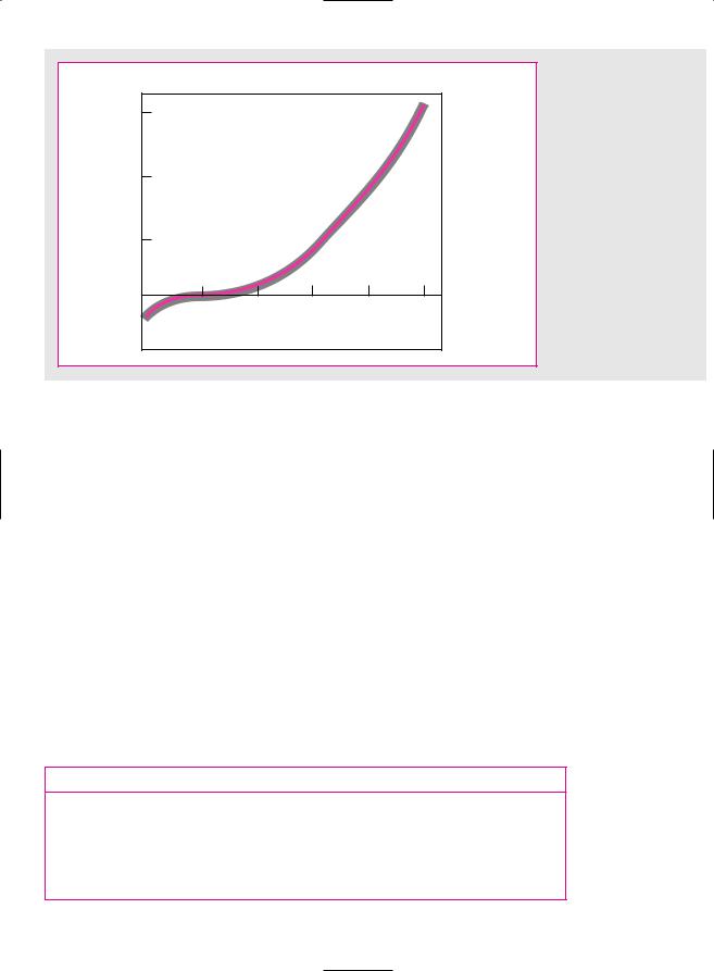
The NPV is negative; therefore, the IRR must be less than 50 percent. In Figure 5.2 we have plotted the net present values implied by a range of discount rates. From this we can see that a discount rate of 28 percent gives the desired net present value of zero. Therefore IRR is 28 percent.
The easiest way to calculate IRR, if you have to do it by hand, is to plot three or four combinations of NPV and discount rate on a graph like Figure 5.2, connect the
Net present value, dollars
+2,000
+1,000 |
|
|
|
|
|
|
|
|
|
|
|
|
IRR = 28 percent |
|
|
|
|
|
|||
0 |
|
|
|
|
|
|
|
|
Discount rate, |
|
20 |
40 |
50 |
60 |
70 |
80 |
90 |
100 |
percent |
||
10 |
||||||||||
F I G U R E 5 . 2
This project costs $4,000 and then produces cash inflows of $2,000 in year 1 and $4,000 in year 2. Its internal rate of return (IRR) is 28 percent, the rate of discount at which NPV is zero.
–1,000
–2,000

98 |
PART I Value |
points with a smooth line, and read off the discount rate at which NPV = 0. It is of course quicker and more accurate to use a computer or a specially programmed calculator, and this is what most financial managers do.
Now, the internal rate of return rule is to accept an investment project if the opportunity cost of capital is less than the internal rate of return. You can see the reasoning behind this idea if you look again at Figure 5.2. If the opportunity cost of capital is less than the 28 percent IRR, then the project has a positive NPV when discounted at the opportunity cost of capital. If it is equal to the IRR, the project has a zero NPV. And if it is greater than the IRR, the project has a negative NPV. Therefore, when we compare the opportunity cost of capital with the IRR on our project, we are effectively asking whether our project has a positive NPV. This is true not only for our example. The rule will give the same answer as the net present value rule whenever the NPV of a project is a smoothly declining function of the discount rate.3
Many firms use internal rate of return as a criterion in preference to net present value. We think that this is a pity. Although, properly stated, the two criteria are formally equivalent, the internal rate of return rule contains several pitfalls.
Pitfall 1—Lending or Borrowing?
Not all cash-flow streams have NPVs that decline as the discount rate increases. Consider the following projects A and B:
|
Cash Flows ($) |
|
|
|
|
|
|
|
|
Project |
C0 |
C1 |
IRR |
NPV at 10% |
A |
–1,000 |
1,500 |
50% |
364 |
B |
1,000 |
–1,500 |
50% |
–364 |
|
|
|
|
|
Each project has an IRR of 50 percent. (In other words, –1,000 1,500/1.50 0 and1,000 – 1,500/1.50 0.)
Does this mean that they are equally attractive? Clearly not, for in the case of A, where we are initially paying out $1,000, we are lending money at 50 percent; in the case of B, where we are initially receiving $1,000, we are borrowing money at 50 percent. When we lend money, we want a high rate of return; when we borrow money, we want a low rate of return.
If you plot a graph like Figure 5.2 for project B, you will find that NPV increases as the discount rate increases. Obviously the internal rate of return rule, as we stated it above, won’t work in this case; we have to look for an IRR less than the opportunity cost of capital.
This is straightforward enough, but now look at project C:
|
|
|
Cash Flows ($) |
|
|
|
|
|
|
|
|
|
|
|
|
|
|
Project |
|
C0 |
C1 |
C2 |
C3 |
IRR |
NPV at 10% |
|
C |
1,000 |
–3,600 |
4,320 |
–1,728 |
20% |
–.75 |
||
|
|
|
|
|
|
|
|
|
3Here is a word of caution: Some people confuse the internal rate of return and the opportunity cost of capital because both appear as discount rates in the NPV formula. The internal rate of return is a profitability measure that depends solely on the amount and timing of the project cash flows. The opportunity cost of capital is a standard of profitability for the project which we use to calculate how much the project is worth. The opportunity cost of capital is established in capital markets. It is the expected rate of return offered by other assets equivalent in risk to the project being evaluated.
CHAPTER 5 Why Net Present Value Leads to Better Investment Decisions Than Other Criteria |
99 |
Net present value, dollars
+60
+40
+20
0 |
|
|
|
Discount rate, |
|
40 |
60 |
80 |
100 percent |
||
20 |
F I G U R E 5 . 3
The NPV of project C increases as the discount rate increases.
–20
It turns out that project C has zero NPV at a 20 percent discount rate. If the opportunity cost of capital is 10 percent, that means the project is a good one. Or does it? In part, project C is like borrowing money, because we receive money now and pay it out in the first period; it is also partly like lending money because we pay out money in period 1 and recover it in period 2. Should we accept or reject? The only way to find the answer is to look at the net present value. Figure 5.3 shows that the NPV of our project increases as the discount rate increases. If the opportunity cost of capital is 10 percent (i.e., less than the IRR), the project has a very small negative NPV and we should reject.
Pitfall 2—Multiple Rates of Return
In most countries there is usually a short delay between the time when a company receives income and the time it pays tax on the income. Consider the case of Albert Vore, who needs to assess a proposed advertising campaign by the vegetable canning company of which he is financial manager. The campaign involves an initial outlay of $1 million but is expected to increase pretax profits by $300,000 in each of the next five periods. The tax rate is 50 percent, and taxes are paid with a delay of one period. Thus the expected cash flows from the investment are as follows:
Cash Flows ($ thousands)
|
|
|
|
|
|
|
Period |
|
|
|
|
|
|
|
|
||
|
0 |
|
1 |
2 |
|
3 |
|
4 |
|
5 |
|
6 |
|
||||
|
|
|
|
|
|
|
|
|
|
|
|
|
|
|
|
|
|
Pretax flow |
–1,000 |
300 |
300 |
300 |
300 |
300 |
|
|
|||||||||
Tax |
|
|
500 |
|
–150 |
|
–150 |
|
–150 |
|
–150 |
–150 |
|
||||
|
|
|
|
|
|
|
|
|
|
|
|
|
|
|
|
|
|
Net flow |
–1,000 |
800 |
150 |
150 |
150 |
150 |
–150 |
|
|||||||||
Note: The $1 million outlay in period 0 reduces the company’s taxes in period 1 by $500,000; thus we enter 500 in year 1.
100 |
PART I Value |
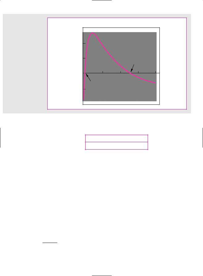
F I G U R E 5 . 4
The advertising campaign has two internal rates of return. NPV 0 when the discount rate is 50 percent and when it is15.2 percent.
Net present value, thousands of dollars 1,500
1,000
500
IRR = 15.2 percent
–25 |
0 |
25 |
50 Discount rate, |
0 |
|
|
percent |
|
|
|
|
IRR = –50 percent |
|
|
|
–500
–1,000
Mr. Vore calculates the project’s IRR and its NPV as follows:
IRR (%) |
NPV at 10% |
50 and 15.2 |
74.9 or $74,900 |
Note that there are two discount rates that make NPV = 0. That is, each of the following statements holds:
NPV 1,000 |
800 |
|
150 |
|
|
150 |
150 |
|
|
|
150 |
|
|
|
|
150 |
0 |
|||||||||||||
|
|
|
|
|
|
|
|
|
|
|
|
|
|
|
|
|
|
|||||||||||||
.50 |
1.502 |
2 |
1.502 |
3 |
1.502 |
4 |
1.502 |
5 |
|
1.502 6 |
||||||||||||||||||||
and |
|
|
|
|
|
|
|
|
|
|
|
|
|
|
|
|
|
|
|
|
|
|
|
|
|
|
|
|
|
|
NPV 1,000 |
|
800 |
|
|
|
150 |
|
|
|
150 |
|
|
|
150 |
|
|
|
|
150 |
|
||||||||||
1.152 |
|
11.1522 2 |
11.1522 3 |
|
1 |
1.1522 4 |
11.1522 5 |
|
||||||||||||||||||||||
150 |
|
|
0 |
|
|
|
|
|
|
|
|
|
|
|
|
|
|
|
|
|
|
|
|
|
|
|
|
|
||
|
|
|
|
|
|
|
|
|
|
|
|
|
|
|
|
|
|
|
|
|
|
|
|
|
|
|
|
|||
11.1522 6 |
|
|
|
|
|
|
|
|
|
|
|
|
|
|
|
|
|
|
|
|
|
|
|
|
|
|||||
In other words, the investment has an IRR of both –50 and 15.2 percent. Figure 5.4 shows how this comes about. As the discount rate increases, NPV initially rises and then declines. The reason for this is the double change in the sign of the cash-flow stream. There can be as many different internal rates of return for a project as there are changes in the sign of the cash flows.4
4By Descartes’s “rule of signs” there can be as many different solutions to a polynomial as there are changes of sign. For a discussion of the problem of multiple rates of return, see J. H. Lorie and L. J. Savage, “Three Problems in Rationing Capital,” Journal of Business 28 (October 1955), pp. 229–239; and E. Solomon, “The Arithmetic of Capital Budgeting,” Journal of Business 29 (April 1956), pp. 124–129.

CHAPTER 5 Why Net Present Value Leads to Better Investment Decisions Than Other Criteria |
101 |
In our example the double change in sign was caused by a lag in tax payments, but this is not the only way that it can occur. For example, many projects involve substantial decommissioning costs. If you strip-mine coal, you may have to invest large sums to reclaim the land after the coal is mined. Thus a new mine creates an initial investment (negative cash flow up front), a series of positive cash flows, and an ending cash outflow for reclamation. The cash-flow stream changes sign twice, and mining companies typically see two IRRs.
As if this is not difficult enough, there are also cases in which no internal rate of return exists. For example, project D has a positive net present value at all discount rates:
|
|
Cash Flows ($) |
|
|
|
|
|
|
|
|
|
|
|
Project |
C0 |
C1 |
C2 |
IRR (%) |
NPV at 10% |
|
D |
1,000 |
–3,000 |
2,500 |
None |
339 |
|
|
|
|
|
|
|
|
A number of adaptations of the IRR rule have been devised for such cases. Not only are they inadequate, but they also are unnecessary, for the simple solution is to use net present value.5
Pitfall 3—Mutually Exclusive Projects
Firms often have to choose from among several alternative ways of doing the same job or using the same facility. In other words, they need to choose from among mutually exclusive projects. Here too the IRR rule can be misleading.
Consider projects E and F:
|
Cash Flows ($) |
|
|
||
|
|
|
|
|
|
Project |
C0 |
C1 |
IRR (%) |
NPV at 10% |
|
E |
–10,000 |
20,000 |
100 |
8,182 |
|
F |
–20,000 |
35,000 |
75 |
11,818 |
|
|
|
|
|
|
|
5Companies sometimes get around the problem of multiple rates of return by discounting the later cash flows back at the cost of capital until there remains only one change in the sign of the cash flows. A modified internal rate of return can then be calculated on this revised series. In our example, the modified IRR is calculated as follows:
1. Calculate the present value of the year 6 cash flow in year 5: PV in year 5 = –150/1.10 = –136.36
2. Add to the year 5 cash flow the present value of subsequent cash flows:
C5 + PV(subsequent cash flows) = 150 – 136.36 = 13.64
3. Since there is now only one change in the sign of the cash flows, the revised series has a unique rate of return, which is 15 percent:
NPV 1,000 |
800 |
|
150 |
|
150 |
|
150 |
|
13.64 |
0 |
1.15 |
1.152 |
1.153 |
1.154 |
1.155 |
Since the modified IRR of 15 percent is greater than the cost of capital (and the initial cash flow is negative), the project has a positive NPV when valued at the cost of capital.
Of course, it would be much easier in such cases to abandon the IRR rule and just calculate project NPV.

102 |
PART I Value |
Perhaps project E is a manually controlled machine tool and project F is the same tool with the addition of computer control. Both are good investments, but F has the higher NPV and is, therefore, better. However, the IRR rule seems to indicate that if you have to choose, you should go for E since it has the higher IRR. If you follow the IRR rule, you have the satisfaction of earning a 100 percent rate of return; if you follow the NPV rule, you are $11,818 richer.
You can salvage the IRR rule in these cases by looking at the internal rate of return on the incremental flows. Here is how to do it: First, consider the smaller project (E in our example). It has an IRR of 100 percent, which is well in excess of the 10 percent opportunity cost of capital. You know, therefore, that E is acceptable. You now ask yourself whether it is worth making the additional $10,000 investment in F. The incremental flows from undertaking F rather than E are as follows:
|
Cash Flows ($) |
|
|
|
|
|
|
|
|
Project |
C0 |
C1 |
IRR (%) |
NPV at 10% |
F–E |
–10,000 |
15,000 |
50 |
3,636 |
|
|
|
|
|
The IRR on the incremental investment is 50 percent, which is also well in excess of the 10 percent opportunity cost of capital. So you should prefer project F to project E.6 Unless you look at the incremental expenditure, IRR is unreliable in ranking projects of different scale. It is also unreliable in ranking projects which offer different patterns of cash flow over time. For example, suppose the firm can take proj-
ect G or project H but not both (ignore I for the moment):
|
|
|
Cash Flows ($) |
|
|
|
|
|
IRR |
NPV |
|
|
|
|
|
|
|
|
|
||
|
|
|
|
|
|
|
|
|
||
Project |
C0 |
C1 |
C2 |
C3 |
C4 |
C5 |
Etc. |
(%) |
at 10% |
|
G |
–9,000 |
6,000 |
5,000 |
4,000 |
0 |
0 |
. . . |
33 |
3,592 |
|
H |
–9,000 |
1,800 |
1,800 |
1,800 |
1,800 |
1,800 |
. . . |
20 |
9,000 |
|
I |
|
–6,000 |
1,200 |
1,200 |
1,200 |
1,200 |
. . . |
20 |
6,000 |
|
|
|
|
|
|
|
|
|
|
|
|
Project G has a higher IRR, but project H has the higher NPV. Figure 5.5 shows why the two rules give different answers. The blue line gives the net present value of project G at different rates of discount. Since a discount rate of 33 percent produces a net present value of zero, this is the internal rate of return for project G. Similarly, the burgundy line shows the net present value of project H at different discount rates. The IRR of project H is 20 percent. (We assume project H’s cash flows continue indefinitely.) Note that project H has a higher NPV so long as the opportunity cost of capital is less than 15.6 percent.
The reason that IRR is misleading is that the total cash inflow of project H is larger but tends to occur later. Therefore, when the discount rate is low, H has the higher NPV; when the discount rate is high, G has the higher NPV. (You can see from Figure 5.5 that the two projects have the same NPV when the discount rate is 15.6 percent.) The internal rates of return on the two projects tell us that at a discount rate of 20 percent H has a zero NPV (IRR 20 percent) and G has a positive
6You may, however, find that you have jumped out of the frying pan into the fire. The series of incremental cash flows may involve several changes in sign. In this case there are likely to be multiple IRRs and you will be forced to use the NPV rule after all.

CHAPTER 5 Why Net Present Value Leads to Better Investment Decisions Than Other Criteria |
103 |
|||||||||||||
|
|
|
|
|
|
|
|
|
|
|
|
|
|
|
|
Net present value, dollars |
|
|
|
|
|
|
|
|
|
|
|||
|
+10,000 |
|
|
|
|
|
|
|
|
|
|
|
|
|
|
|
|
|
|
|
|
|
|
|
|
|
|
|
|
|
|
|
|
|
|
|
|
|
|
|
|
|
|
|
|
+6,000 |
|
|
|
|
|
|
|
|
|
|
|
|
|
|
|
|
|
|
|
|
|
|
|
|
|
|
|
|
|
+5,000 |
|
|
|
|
|
33.3 |
|
|
|
|
|
|
|
|
|
|
|
|
|
|
|
|
|
|
|
|||
|
|
|
|
|
|
|
|
|
|
|
|
|
||
|
|
|
|
|
|
|
40 |
50 |
Discount rate, |
|
|
|||
|
0 |
|
|
|
|
|
|
|
|
|
|
|
|
|
|
10 |
20 |
30 |
|
|
Project G |
percent |
|
|
|||||
|
|
|
|
|
|
|||||||||
|
|
|
|
|
|
|
|
|
|
|
|
|
|
|
|
|
15.6 |
|
|
|
|
|
|
|
|
|
|
||
|
–5,000 |
|
|
|
|
|
|
|
|
Project H |
|
|
|
|
|
|
|
|
|
|
|
|
|
|
|
||||
|
|
|
|
|
|
|
|
|
|
|
|
|
|
|
|
|
|
|
|
|
|
|
|
|
|
|
|
|
|
F I G U R E 5 . 5
The IRR of project G exceeds that of project H, but the NPV of project G is higher only if the discount rate is greater than 15.6 percent.
NPV. Thus if the opportunity cost of capital were 20 percent, investors would place a higher value on the shorter-lived project G. But in our example the opportunity cost of capital is not 20 percent but 10 percent. Investors are prepared to pay relatively high prices for longer-lived securities, and so they will pay a relatively high price for the longer-lived project. At a 10 percent cost of capital, an investment in H has an NPV of $9,000 and an investment in G has an NPV of only $3,592.7
This is a favorite example of ours. We have gotten many businesspeople’s reaction to it. When asked to choose between G and H, many choose G. The reason seems to be the rapid payback generated by project G. In other words, they believe that if they take G, they will also be able to take a later project like I (note that I can be financed using the cash flows from G), whereas if they take H, they won’t have money enough for I. In other words they implicitly assume that it is a shortage of capital which forces the choice between G and H. When this implicit assumption is brought out, they usually admit that H is better if there is no capital shortage.
But the introduction of capital constraints raises two further questions. The first stems from the fact that most of the executives preferring G to H work for firms that would have no difficulty raising more capital. Why would a manager at IBM, say, choose G on the grounds of limited capital? IBM can raise plenty of capital and can take project I regardless of whether G or H is chosen; therefore I should not affect the choice between G and H. The answer seems to be that large firms usually impose capital budgets on divisions and subdivisions as a part of the firm’s planning and control system. Since the system is complicated and cumbersome, the
7It is often suggested that the choice between the net present value rule and the internal rate of return rule should depend on the probable reinvestment rate. This is wrong. The prospective return on another independent investment should never be allowed to influence the investment decision. For a discussion of the reinvestment assumption see A. A. Alchian, “The Rate of Interest, Fisher’s Rate of Return over Cost and Keynes’ Internal Rate of Return,” American Economic Review 45 (December 1955), pp. 938–942.

104 |
PART I Value |
budgets are not easily altered, and so they are perceived as real constraints by middle management.
The second question is this. If there is a capital constraint, either real or selfimposed, should IRR be used to rank projects? The answer is no. The problem in this case is to find that package of investment projects which satisfies the capital constraint and has the largest net present value. The IRR rule will not identify this package. As we will show in the next section, the only practical and general way to do so is to use the technique of linear programming.
When we have to choose between projects G and H, it is easiest to compare the net present values. But if your heart is set on the IRR rule, you can use it as long as you look at the internal rate of return on the incremental flows. The procedure is exactly the same as we showed above. First, you check that project G has a satisfactory IRR. Then you look at the return on the additional investment in H.
|
|
|
Cash Flows ($) |
|
|
|
|
IRR |
NPV |
|
|
|
|
|
|
|
|
|
|
||
|
|
|
|
|
|
|
|
|
||
Project |
C0 |
C1 |
C2 |
C3 |
C4 |
C5 |
Etc. |
(%) |
at 10% |
|
H–G |
0 |
–4,200 |
–3,200 |
–2,200 |
1,800 |
1,800 |
|
15.6 |
5,408 |
|
|
|
|
|
|
|
|
|
|
|
|
The IRR on the incremental investment in H is 15.6 percent. Since this is greater than the opportunity cost of capital, you should undertake H rather than G.
Pitfall 4—What Happens When We Can’t Finesse the Term Structure of Interest Rates?
We have simplified our discussion of capital budgeting by assuming that the opportunity cost of capital is the same for all the cash flows, C1, C2, C3, etc. This is not the right place to discuss the term structure of interest rates, but we must point out certain problems with the IRR rule that crop up when short-term interest rates are different from long-term rates.
Remember our most general formula for calculating net present value:
NPV C0 |
|
|
C1 |
|
C2 |
|
|
C3 |
… |
|
|
11 r2 2 2 |
|
r3 2 3 |
|||||
|
1 |
r1 |
11 |
|
|||||
In other words, we discount C1 at the opportunity cost of capital for one year, C2 at the opportunity cost of capital for two years, and so on. The IRR rule tells us to accept a project if the IRR is greater than the opportunity cost of capital. But what do we do when we have several opportunity costs? Do we compare IRR with r1, r2, r3, . . .? Actually we would have to compute a complex weighted average of these rates to obtain a number comparable to IRR.
What does this mean for capital budgeting? It means trouble for the IRR rule whenever the term structure of interest rates becomes important.8 In a situation where it is important, we have to compare the project IRR with the expected IRR (yield to maturity) offered by a traded security that (1) is equivalent in risk to the project and (2) offers the same time pattern of cash flows as the project. Such a comparison is easier said than done. It is much better to forget about IRR and just calculate NPV.
8The source of the difficulty is that the IRR is a derived figure without any simple economic interpretation. If we wish to define it, we can do no more than say that it is the discount rate which applied to all cash flows makes NPV = 0. The problem here is not that the IRR is a nuisance to calculate but that it is not a useful number to have.

CHAPTER 5 Why Net Present Value Leads to Better Investment Decisions Than Other Criteria |
105 |
Many firms use the IRR, thereby implicitly assuming that there is no difference between short-term and long-term rates of interest. They do this for the same reason that we have so far finessed the term structure: simplicity.9
The Verdict on IRR
We have given four examples of things that can go wrong with IRR. We spent much less space on payback or return on book. Does this mean that IRR is worse than the other two measures? Quite the contrary. There is little point in dwelling on the deficiencies of payback or return on book. They are clearly ad hoc measures which often lead to silly conclusions. The IRR rule has a much more respectable ancestry. It is a less easy rule to use than NPV, but, used properly, it gives the same answer.
Nowadays few large corporations use the payback period or return on book as their primary measure of project attractiveness. Most use discounted cash flow or “DCF,” and for many companies DCF means IRR, not NPV. We find this puzzling, but it seems that IRR is easier to explain to nonfinancial managers, who think they know what it means to say that “Project G has a 33 percent return.” But can these managers use IRR properly? We worry particularly about Pitfall 3. The financial manager never sees all possible projects. Most projects are proposed by operating managers. Will the operating managers’ proposals have the highest NPVs or the highest IRRs?
A company that instructs nonfinancial managers to look first at projects’ IRRs prompts a search for high-IRR projects. It also encourages the managers to modify projects so that their IRRs are higher. Where do you typically find the highest IRRs? In short-lived projects requiring relatively little up-front investment. Such projects may not add much to the value of the firm.
5.4 CHOOSING CAPITAL INVESTMENTS WHEN RESOURCES ARE LIMITED
Our entire discussion of methods of capital budgeting has rested on the proposition that the wealth of a firm’s shareholders is highest if the firm accepts every project that has a positive net present value. Suppose, however, that there are limitations on the investment program that prevent the company from undertaking all such projects. Economists call this capital rationing. When capital is rationed, we need a method of selecting the package of projects that is within the company’s resources yet gives the highest possible net present value.
An Easy Problem in Capital Rationing
Let us start with a simple example. The opportunity cost of capital is 10 percent, and our company has the following opportunities:
|
Cash Flows ($ millions) |
|
|||
|
|
|
|
|
|
Project |
C0 |
C1 |
C2 |
NPV at 10% |
|
A |
–10 |
30 |
5 |
21 |
|
B |
–5 |
5 |
20 |
16 |
|
C |
–5 |
5 |
15 |
12 |
|
|
|
|
|
|
|
9In Chapter 9 we will look at some other cases in which it would be misleading to use the same discount rate for both short-term and long-term cash flows.

106 |
PART I Value |
All three projects are attractive, but suppose that the firm is limited to spending $10 million. In that case, it can invest either in project A or in projects B and C, but it cannot invest in all three. Although individually B and C have lower net present values than project A, when taken together they have the higher net present value. Here we cannot choose between projects solely on the basis of net present values. When funds are limited, we need to concentrate on getting the biggest bang for our buck. In other words, we must pick the projects that offer the highest net present value per dollar of initial outlay. This ratio is known as the profitability index:10
net present value
Profitability index
investment
For our three projects the profitability index is calculated as follows:11
|
Investment |
NPV |
Profitability |
Project |
($ millions) |
($ millions) |
Index |
|
|
|
|
A |
10 |
21 |
2.1 |
B |
5 |
16 |
3.2 |
C |
5 |
12 |
2.4 |
|
|
|
|
Project B has the highest profitability index and C has the next highest. Therefore, if our budget limit is $10 million, we should accept these two projects.12
Unfortunately, there are some limitations to this simple ranking method. One of the most serious is that it breaks down whenever more than one resource is rationed. For example, suppose that the firm can raise only $10 million for investment in each of years 0 and 1 and that the menu of possible projects is expanded to include an investment next year in project D:
|
|
Cash Flows ($ millions) |
|
|
||
|
|
|
|
|
|
|
Project |
|
C0 |
C1 |
C2 |
NPV at 10% |
Profitability Index |
A |
–10 |
30 |
5 |
21 |
2.1 |
|
B |
|
–5 |
5 |
20 |
16 |
3.2 |
C |
|
–5 |
5 |
15 |
12 |
2.4 |
D |
0 |
–40 |
60 |
13 |
0.4 |
|
|
|
|
|
|
|
|
One strategy is to accept projects B and C; however, if we do this, we cannot also accept D, which costs more than our budget limit for period 1. An alternative is to
10If a project requires outlays in two or more periods, the denominator should be the present value of the outlays. (A few companies do not discount the benefits or costs before calculating the profitability index. The less said about these companies the better.)
11Sometimes the profitability index is defined as the ratio of the present value to initial outlay, that is, as PV/investment. This measure is also known as the benefit–cost ratio. To calculate the benefit–cost ratio, simply add 1.0 to each profitability index. Project rankings are unchanged.
12If a project has a positive profitability index, it must also have a positive NPV. Therefore, firms sometimes use the profitability index to select projects when capital is not limited. However, like the IRR, the profitability index can be misleading when used to choose between mutually exclusive projects. For example, suppose you were forced to choose between (1) investing $100 in a project whose payoffs have a present value of $200 or (2) investing $1 million in a project whose payoffs have a present value of $1.5 million. The first investment has the higher profitability index; the second makes you richer.