

Digital Image
Processing
Lecture 6: Image
GeometryProf. Charlene Tsai

Geometric Operations
Scale - change image content size
Rotate - change image content orientation
Reflect - flip over image contents
Translate - change image content position
Affine Transformation
general image content linear geometric transformation
2

Geometric transformations
Geometric transformations are common in computer graphics, and are often used in image analysis.
Geometric transforms permit the elimination of geometric distortion that occurs when an image is captured.
If one attempts to match two different images of the same object, a geometric transformation may be needed.
Examples?
3

Geometric Transformations
A geometric transform consists of two basic steps ...
Step1: determining the pixel co-ordinate transformation
mapping of the co-ordinates of the moving image pixel to the point in the fixed image.
T(x,y) |
(x,y) |
Fixed Image |
Moving Image |
|
4 |
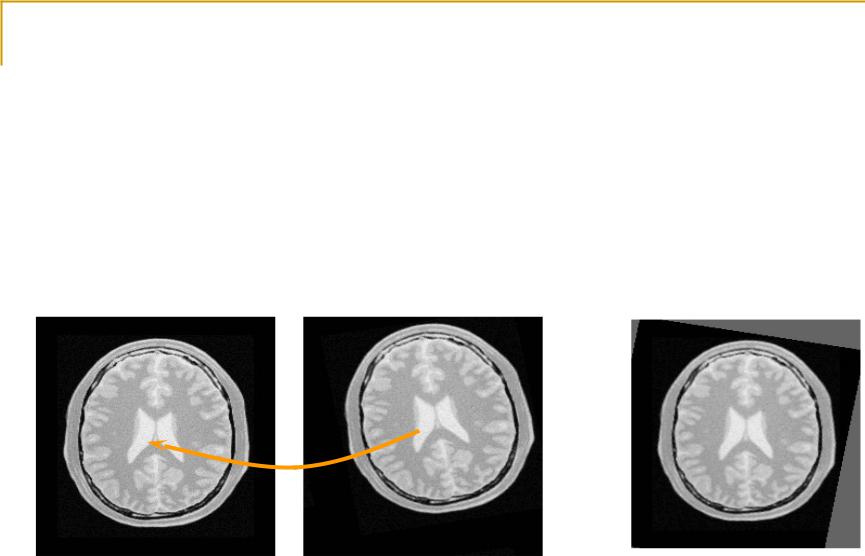
Geometric transformations
Step2: determining the brightness of the points in the digital grid of the transformed image.
brightness is usually computed as an interpolation of the brightnesses of several points in the neighborhood.
T(x,y) |
(x,y) |
Fixed Image |
Moving Image |
xformed Moving Image |
|
|
|
|
|
We’ll discuss step 2 first. |
|
5 |
|

x1, x2, x3, x4 are original points
X’i are
new points
6

Another Example
Interpolation on an image (4x4 -> 8x8) after scaling
Open circle: Original image pixel
 Closed circle:
New pixels
7

Interpolation: Nearest
1-D |
We assign f (xi’ )=f (xj) |
|||
|
|
|||
|
|
xj is the original point closest to x |
||
|
|
|
The original function values |
|
|
|
|
The interpolated values |
|
2-D |
|
x’ |
||
|
Origina |
|
|
|
|
l point |
|
Interpolated |
|
|
|
|
point |
|
|
|
y’ |
|
|
|
|
|
|
|
|
|
|
||
setting the pixel value on interpolated point to the pixel of closet image point

Interpolation: Linear (1D)
General idea:
original function values |
To calculate the |
interpolated values |
interpolated |
|
f(x2)-f(x1) |
9

Interpolation: Linear (2D)
How a 4x4 image would be interpolated to produce an 8x8 image?
f x, y' f x, y 1 1 f x, y
4 original pixel values
f x 1, y' f x 1, y 1 1 f x 1, y
one interpolated pixel value
Along the y’ column we have
f x', y' f x 1, y' (1 ) f (x, y')
10