Добавил:

maiminh06 Опубликованный материал нарушает ваши авторские права? Сообщите нам.

Вуз:

Национальный исследовательский ядерный университет (МИФИ)

Предмет:

[НЕСОРТИРОВАННОЕ]

Файл:

Vol D - 1990 (ocr) ELECTRICAL SYSTEM & EQUIPMENT

.pdf

Скачиваний:

Добавлен:

17.07.2023

Размер:

30.18 Mб

Скачать

☆

<<< < Предыдущая 61 62 63 64 65 66 67 68 69 70 71 7273 / 10673 74 75 76 77 78 79 80 81 82 83 84 85 > Следующая >>>

Radio systems

practice, this is the value of impedance which, when

From which P = 4SP/(S

1) 2

terminating any length of the cable, will produce an

ut impedance of the game value.

For VSWR = S = 1.5, P = 0.96 P m , i.e., for a

n For a perfect match between the coaxial cable and

VSWR = 1.5, 9607o of the power that would be

the antenna impedances, there is no reflected signal

delivered to a matched load

is delivered to the un-

from the antenna/coaxial cable connection and there-

matched antenna; this is equivalent to a

loss of 10 log

fore no standing wave, i.e., I E mu ,' = I

and the

0.96 = 0.2 dB.

R = 1.

From Fig 8.21, it can be seen that the bandwidth

For a \,alue of antenna impedance which is less or

between the 1.5 VSWR points for a

VHF

version

[tie:1[er than the characteristic impedance of the coaxial

of the CAT 80 antenna is approximately 2.5

MHz.

ble

he vsWR will be greater than 1.

From Fig 8.22, the bandwidth of a CAT 460 UHF an-

I Emax 1

I F11+1Erl

tenna is approximately 22 MHz. The VSWR/frequency

VSWR —

(8.22)

graphs for the CAT 80 and the CAT 460 antennas

I Emm I

I Er I —

E I

show that, at the design frequency for the antennas,

the VSWR is approximately 1.15 and that the VSWR

0. here Er

voltage of the forward travelling wave

changes with frequency.

The power handling capability of the antenna will

= voltage of the reflected wave

depend on the maximum RF output of the transmitter.

— 0, VSWR = 1

when E r

For a CAT type antenna, the maximum input power

For VSWR

1.5, I E max 1 = 1.21 Ef I

is 150 W, which is well above any transmitter output

and I E m m = 0.8 I Ef I

used for a power station radio system.

The input impedance of an antenna is specified for

To appreciate the meaning of VSWR

1.5, it is useful

the design frequency and will vary between the VSWR

to calculate the impedance of the load of the antenna

1.5 points of the antenna bandwidth. For power station

..ompared with a coaxial cable characteristic of 50 0.

systems, the design impedance is usually 50 0: this

Co do this, the following equations can be used:

varies between 50 and 75 0 over the design bandwidth

Z — Zo

of the antenna.

(8.23)

The mounting arrangement will depend on the type

Z + Zo

of antenna chosen. The mounting arrangements for a

CAT type colincar antenna suitable for masthead

where

voltage reflection coefficient

mounting are shown in Fig 8.23.

Z = antenna impedance, 0

Zo = characteristic impedance of the coaxial cable, 0

The modulus of the voltage reflection coefficient						e I
o determined from the VSWR:
	Is -I I			I z - zo I	(8.24)
	I s +			Iz+ zoi	(8.24)
	I s +			Iz+ zoi
here S = VSWR = 1.5 and if Zo = 50 0
I z - 501		0.5	giving 1 Z1 = 75
then			giving 1 Z1 = 75
1 Z +501		2.5
The power delivered to		the antenna at a VSWR =				1.5
Lan be calculated using:
Mismatch loss =				P rn /P
" h ere Pm + power delivered to a matched load
P = power delivered to the antenna

3.0 —

.0000000. 44,

2 0 —

1 0 —

2.0 —

>1 5—

1 0		79	80	81	82	83	[	85
78							84

FREQUENCY MHz

P in
P in		(s + 1) 2
	- Q1 2	4S	Fm. 8.21 Gain and VSWR curves for a Philips VHF
			CAT 80 antenna

687

Telecommunications	Chapter 8

cc 1 5

•J")

TYPE NO	FREQUENCY SAND MHz
TYPE NO	FOR 1 5. 1 MAX VSWR)

CAT 390	380	- 396
CAT 400	396	- 412
CAT 420	412.430
CAT 440	430	- 450
CAT 460	450	•470

Fib. 8.22 VSWR curves for Philips UHF CAT antennas

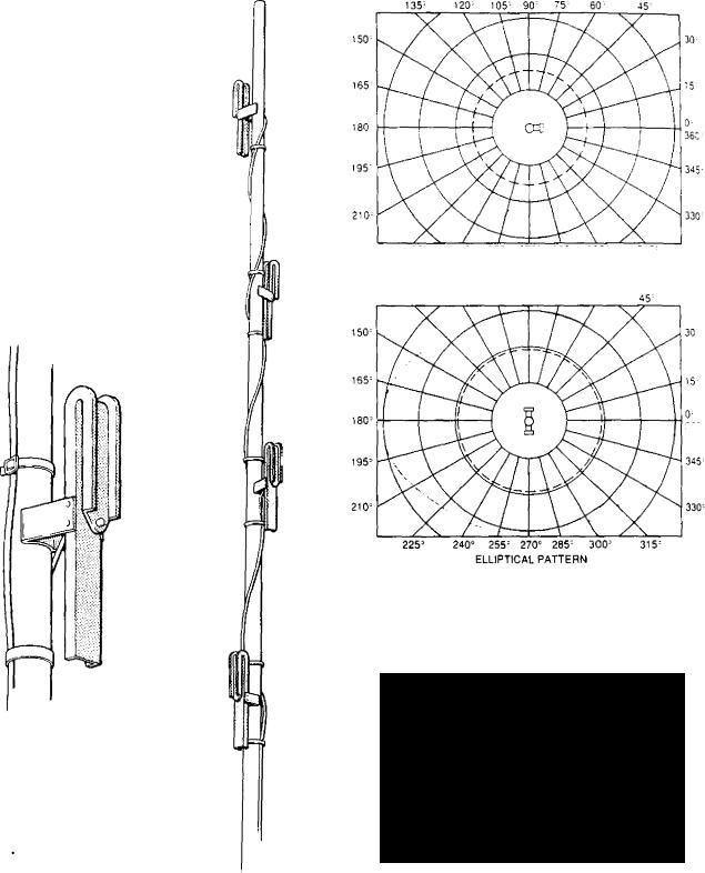
Folded dipole antennas which can be used for both VHF and VHF systems are supplied with a mounting boom. Figure 8.24 shows a typical folded dipole antenna, the Philips Telecom Type ANSDH, which has a 38 mm diameter mounting boom. Figure 8.25 shows the typical mounting crossover clamps used to attach the boom to a mast. The mast fixing arrangement must be capable of withstanding a wind loading of 160 km/h. For power station external antennas the mast is usually clamped to a suitable wall or to metal girder sections at two points along its length.

The Type ANSDH 460, or similar, is used as an internal antenna for UHF on-site systems. When used in this way, the mounting boom can be supplied with a wall bracket and enough boom length to allow the wall to antenna spacing to be adjusted between 3/16 and 1/4 of a wavelength. The spacing should be adjusted for maximum radiation.

Figure 8.26 shows the effect of the proximity of a mast on the polar diagram of the antenna. In this case, a boom length of 1 wavelength or more will give the best omnidirectional pattern.

When designing/installing antenna systems, it is necessary to reduce the coupling between transmitter and receiver antennas used for a common two-frequency simplex channel and between antennas of different channels. This is necessary to prevent unwanted signal levels appearing at the output of transmitters and the input of receivers, which could result in intermodulation interference.

Figure 8.27 shows the relationship between isolation in decibels and the vertical separation between the antennas, while Fig 8.28 shows the relationship between isolation in decibels and horizontal separation between the antennas.

Comparison of the two figures shows that the vertical separation is more effective than the horizontal, e.g., at 450 MHz, 35 dB isolation can be obtained by vertical separation of 0.6 m or by a horizontal separation of 4.2 m.

Irs line Olt set Masillead Camp

Parallel Clamp

Parallel Clamps

AG. 8.23 Clamping arrangements for CAT antennas

688

Radio systems

i(,. 8.24 Folded dipole antenna, Philips type ANSDH

8.6.2Typical antenna arrangements

In the past a typical external antenna arrangement for rower stations comprised a mast with folded dipoles for He transmitter and a common omnidirectional high Lia m antenna for the receivers. The high gain receive Antenna was mounted at the top of the mast and the bolded dipoles 3 m below.

Flgures 8.24 and 8.29 show a typical folded dipole and the dipole characteristics: Figs 8.30 and 8.31 illustrate a typical high gain omnidirectional antenna (Philips Type ANSA) and its associated characteristics. The high gain antenna consists of four vertical dipoles iflaunted on a 38 mm support tube. The dipoles are

FIG. 8,25 Typical crossover/parallel clamps for boommounted folded dipoles

fed in a suitable phase relationship by a matching harness which is attached to the support tube. Gain in the direction of maximum radiation is approximately 5 dB relative to a half-wave dipole.

Figure 8.31 shows the H-plane radiation patterns which can be obtained by re-arranging the dipoles, e.g., all four dipoles can be mounted on the same side of the support tube to provide extra gain in one direction, resulting in a gain of 8.5 dB.

Figure 8.32 shows the E-plane polar diagram for the high gain antenna. The lobes showing that the direction of maximum gain radiate horizontally. This would result in poor on-site cover from an antenna mounted on a high building. For a high gain antenna mounted on the roof of a turbine hall or boiler house, some E-plane tilt is required to obtain on-site cover. E-plane

689

Telecommunications		Chapter 8

SUPPORTING STRUCTURE DIAMETER IN WAVELENGTHS

ow* at Mkt

					2k

	4	2
	4	2	4
			4

ANTNNA SPACING TO NEAREST SUPPORT STRUCTURE				NOTE: 2ND CONCENTRIC CIRCLE REPRESENTS
ANTNNA SPACING TO NEAREST SUPPORT STRUCTURE				RADIATOR PATTERN OF ANTENNA IN FREE SPACE

FIG. 8.26 Effect of spacing on the radiation pattern

1 0

20 -

Jo -

ISOLATION. dB

FIG. 8.27 Isolation by vertical separation of antennas

1 0

20—

30 —

100

SEPARATION BETWEEN ANTENNAS. m

tilts of 5° and 10 ° can be obtained electrically by fitting
special matching harnesses which comprise tuned co-	FIG. 8.28 Isolation by horizontal separation
axial cable elements.	of antennas

690

ii Th

Radio systems

															WiND								MiNIMUM , DISTANCE
		jEREOLJECY!													LOADING								SPACING • BETWEEN
		'HAND									1	W EJGH T			AT 193 km ir							' FROM					! CENTFIESOF
		l! FCR	5'				! LENGTH					W EJGH T			I 1 20 MP"						1		50M en.				STACKED
--							! LENGTH					■ LESS E3OCM			ANTENNA ONLY							I	MAST				, DIPOLES
--									mm											kg					mm
									mm											kg					mm
								2^.60					2						58						364			3
			2-23					123.0				25																2 -

								'		€5			24
		— 25						'		€5			24	7						2								2 5 _
			"		'42;							22		' 53									553					24	I
445 1						5					2		)						Si			I	'27					-1 5
															BOOM D 45 Kg PER

																5
																cc

																	1 0
	55 60 65 70 75 80 85 90																1 0

																		380			400		420			440		460	480
				MHz																				MHz

FIG. 8.29 Folded dipole characteristics

T o ts have shown that the circular E-plane polar trarn of a half-wave dipole can give superior on-site er to a high gain antenna. Alternatively, an antenna

.: , t.nvement consisting of two folded dipoles mounted i c above the other in a cruciform arrangement with i• planes parallel and horizontal, will produce a field 1 1 ,i ■ ine a circular polarity (i.e., both vertical and hori- ini tial) directed downward. This paging system type ,Littenna gives localised site cover more suitable for

;, ,mer stations. An antenna of this type is shown in

8.33which also illustrates the depressed E-plane po[ar diagram sometimes referred to as an 'umbrella'

characteristic. This is far more suitable for on-site t. I IF radio systems where the antenna is mounted at level on one of the power station buildings.

In designing the antenna system for a power sta- 'ion, it is necessary to consider the cover required, the on which the antennas are to be mounted and ai ti-plane polar diagrams of the proposed antennas.

it umber of folded dipole antennas located at different around the site and mounted at low level zi‘e better on-site cover than one high gain antenna.

[ lie adoption of multiple fixed station operation, to handportable RF outputs to be reduced, also takes the use of multiple antennas mounted at lower

k‘els more acceptable.

The arrangement that is eventually adopted will be

.rerrnined by the size and complexity of the layout yl, power st.ation buildings, the RF output from the :: indportables, that can be permitted without causing :na :ceptable levels of RFI to control and instrumen- !mion equipment and the cost advantages which will

from use of a radio communications system.

8.6.3 Radiating cable (leaky feeder)

Radiating cable is specially designed coaxial cable which a loosely braided or slotted solid copper outer con-

ductor. The hole in the braid or solid copper outer conductor creates three mutually perpendicular elements of RF field; one element parallel with the cable, one tangential with the cable and the other perpendicular to the cable. For RF transmitted from the cable, the latter element is perpendicular in the direction leaving the cable. For RF received from a handportable transmitter, a similar field arrangement is created by the holes but in this case the perpendicular element is directed into the cable.

The effectiveness of the radiating cable is measured as a coupling loss. The coupling loss is measured by mounting a dipole 3 m or 6 m away from the cable such that the dipole elements are parallel with the radiating cable. The dipole is connected to a matched, calibrated, measuring RF receiver. One end of the radiating cable is connected to a calibrated RF transmitter and the other end to a matched resistive load.

The transmitter is set to a suitable RF input power to the radiating cable which produces a readable signal on the calibrated receiver connected to the dipole.

The overall loss comprises the attenuation due to the radiating cable (cable loss CD) between the input connections and the cable opposite the receiving dipole, and the coupling loss (CL) between the radiating cable and the dipole.

Table 8.4 shows typical cable attenuation and coupling losses for a BICC radiating cable Type T3537 and an Andrew Antenna radiating cable Type Radiax R42R.

Figure 8.34 shows a fixed station transceiver connected to a length of radiating cable through a coupling interface (CI).

The maximum attenuation (MAF) between a fixed station transmitter and a handportable receiver is determined by subtracting the minimum operational power required at the input to the receiver from the output power of the fixed station transmitter. These powers

691

Telecommunications

Chapter 8

135'

120'

105

90=

60'

150

165

180

0•

195 -

345•

210-

330

225'

240' 255' 270' 285 -

300:

315

OFF-SET PATTERN

135'

120"

105' 90

75 -

60'

150'

165'

180'-

360 .

195'

345'

210'

330'

225'

240° 255270' 285' 300'

315'

ELLIPTICAL PATTERN

Flo. 8.31 H-plane polar diagrams for high gain antenna Philips type ANSA

135'		120' 105' 90'	75' 60'	45'
150'					30'

180'				360'
180'	rata4W#*Aim			360'
165'				15'
					Or


195'		ts.		345:
210°		I		330'
210°				330'
	225' 240' 255 270' 285' 300"		315'

FIG. 8.30 Philips type ANSA high gain antenna

are usually quoted in decibels with respect to 1 W

(dBW), i.e., dBW = 10 log	Measured power
		(or 10 log

	One watt
measured power, in watts)

FIG. 8.32 E - plane polar diagram for high gain antenna Philips type ANSA

The maximum attenuation (MAH) between a handportable transmitter and a fixed station receiver is found in a similar manner.

692

distribution loss can be

Radio systems

In order to calculate MAF and MAH it is necessary to determine the losses involved at the handportable.

In both receive directions, although the minimum receiver sensitivity is of the order of 0.5 V pd (1 12 V Els/IF, see Fig 8.36), a minimum operational sensitivity of between 2 and 5 AV EMF would normally be used to design the system.

The body proximity loss ( BP) for the handportable is not necessarily the same for transmit and receive. This is because during transmit the handportable is held at head level and during the receipt of a call it could be attached to a belt or in a pocket. This could result in a BP of up to 3 dB for transmit and up to 6 dB for receive.

For a receiver with an operational sensitivity of 2.5 Pd ( — 129 dBW), a fixed station transmit power of 25 W (14 dBW) and a handportable transmit power of

0.5 W ( — 3 dBW) into the antenna, N1AF and MAH can be calculated as follows:

MAF = 14 — (-129) =	143 dB
MAH = —3 — (-129) — 126 dB
Using these values for MAF and	NIAH the cable

calculated from the following equations, see also Fig 8.34.

MAF = CI + CD + CL + RD + BPL + AL (8.25)

MAH = AL + BPL + CL + RD + CI

(8.26)

where AL = antenna loss

BPL = body proximity loss CD = cable distribution loss CI cable interface loss

RD = Rayleigh distribution loss

FIG. 8.33 Paging type antenna — Jaybeam type 7395

693

because an amplifier

(CI) could be 3 dB

normally be taken as the value to carry out

Telecommunications

Chapter 8

TABLE 8.4

Typical cable attenuation and coupling losses

Radiating cable

Nominal

Frequency

Attenuation

Coupling

diameter

dB/I00 m

loss

BICC 13537

13 mm

85 X1Hz

2.8

64 dB at 3 m

50 ,:? ..- able

67 dB at 6 m

( Aperr Lirecl ape)

450 MHz

6.8

7 -1 dB at 3 m

77 dB at 6 m

Andrews 1(4- 2R

13 mm

55 MHz

3.6

69 dB at 6 m

(Slotted screen)

7 5 dB at 6 m

450 X1Flz

1 0.5

FIXED STATION

RADIATING CABLE

RADIO

TRANSMITTER

CdBW

5011 TERmiNATLNG

RADIO

RESISTOR

RECEIVER

CL . RD

ANTENNA LOSS

BPL - BODY PROXIMITY LOSS

= CABLE DISTRIBUTION LOSS

= CABLE INTERFACE LOSS

1-( ANDPORTABLE

- COUPLING LOSS

RAYLEIGH DiSTRuBITON LOSS

FIG. 8.34 Calculation of maximum cable distribution loss

Since N4AH is smaller than MAF the former would the calculation of CD. However, in practice, since the cable inter-

face loss (CI) and 13P loss differ for the transmit and receive directions it is prudent to calculate CD for both

directions.

The cable interface loss in the transmit direction for a single-transmitter/receiver arrangement or up to 6 dB for a 5-transmitter arrangement. In the receive direction,

could be used before the receiver, the Cl would be dependent on the gain of the amplifier used. A typical value for CI would be — 10 dB (i.e., a gain of 10 dB).

The Rayleigh Distribution loss (RD) covers the losses experienced by a handportable while on the move. The loss is due to multiple path reflections causing variation in the received signal due to the complex summing of signals received from the radiating cable direct, and signals reflected from the walls, ceiling, floors and plant.

As the receiver moves through the field, the signal strength plotted against distance will reveal a standing

wave created in space with the signal strength following a Rayleigh probability distribution. A typical standing wave is shown in Fig 8.35. It can be seen that the signal strength varies between the minimum of 10 dB to the maximum of 20 dB, i.e., a total variation loss of 10 dB.

LINEAR DISTANCE. X 2

Ftc. 8.35 Signal intensity plotted against distance in a multipath environment (Rayleigh Distribution)

694

(b) Showing how a

									Radio systems

Referring to Fig 8.36 (a), it can be seen that in order
t o obtain a				receiver input of 2.5 V pd the EMF ex-			ORTHOGONAL
ted by the antenna from the radiating field must							ORTHOGONAL
, rac							CONDUCTING
, rac	I N, i.e., 126 dBW.						PLANE
In the transmit ditection, Fig 8.36 (b) shows that
.t cransini[f,:r				output of 1 W is necessary in order to
.t cransini[f,:r
,ftilOcr 0.5 N,1 into the antenna.
,ftilOcr 0.5 N,1 into the antenna.
Sin ,:e [he radiating cable coupling loss is specified as
		bet‘een he cable and a two-element hall-wave
Ji ro le, the handportable antenna loss (AL) must be					(a)
			\\,ith respect to a dipole. The antenna is either
,t quarter			wavelength monopole or helical antenna.
FiI' Ve			8.37 shows the relationship between a mono-
pole lia%..ing a practical ground plane and a dipole. The
	parallel to the ground plane is shown to be —3 dB						CONDUCTING
ith respect to a dipole.							CONDUCTING
ith respect to a dipole.								PLANE
For a handportable the ground plane is likely to be
,ornplex and difficult to determine. The value of body						Ei2
pro \ imity			loss ( BP) includes any loss due to a poor			Ez2
round plane.						Ez2
round plane.
Tables 8.5 and 8.6 identify typical handportable
,i menna losses obtained in practice.					(b)
Typical values for each of the losses required in					(b)
Typical values for each of the losses required in
oricr	to determine the maximum cable distribution
are as follows:
11		= 3 dB
BPL = 3 dB for transmitter and 6 dB for receiver						10ADIAMETER
CD		= to be calculated				10ADIAMETER
CD		= to be calculated			90•	GROUND-PLANE
Cl		- 3 dB for a single transmitter and up to							iNFINITE
Cl		- 3 dB for a single transmitter and up to						GROUND-PLANE

6 dB for 5 transmitters

: a.Ea NP T POWER	2			x 50	W
-		2	x	1
- V			x	so W

V p d 2 pV

RECEIVER

NPLIT IMPEDANCE

0 5W DELIVERED TO THE ANTENNA

8.36Calculation of receiver input powers

(c)

FIG. 8.37 Effects of ground plane on a monopole antenna

(a) Dipole element into which a thin conducting sheet has been inserted.

voltage generator can be split so that connection can be made to the conducting plate to form two

identical and separate monopoles, each having a feed point i mpedance half that of a dipole.

(c) Free space radiation patterns of X/4 monopoles over perfectly conducting ground planes of various diameters. The infinite ground plane shows a 3 dB gain over a dipole a 0 0 elevation angle, but any finite ground plane will exhibit a 3dB loss.

CI = — 10 dB (gain) for receiver

CL = 80 dB

MAF = 143 d13

MAH = 126 dll

595

Telecommunications	Chapter 8

From Equation (8.25)

CD = MAF - CI CL - RD - BPL - AL

=143 - 6 - 80 - 10 - 6 - 3

=38 dB

From Equation (8.26)

CD =MAFIAL BPL - CL - RD - Cl

=126- 3 - 3 - SO - 10 - (-10)

=40 dB

For Andrews (R4-2R) type radiating cable and an operating frequency of 450 MHz, 38 dB is equivalent to a length of 362 in of cable which is not sufficient for use in a complex antenna system required for a power station.

However, if the transmitter is connected to the centre of the radiating cable, as shown in Fig 8.38, the radiating cable either side of the power splitter can have a maximum loss of:

38 - (3.5 + 3.5) = 31.0 dB

Since at 450 MHz Andrews (R4-2R) radiating cable has an attenuation of 10.5 dB/100 m, the length of cable on either side of the power splitter can be 31.0/

TERMINATING

RESISTOR

0.105 = 295 m. Thus the total amount of radiating cable that can be used is increased to 10 + 2 x 295 = 600 m.

This procedure can be repeated to produce a complex radiating cable and internal antenna system (see Fig 8.39).

8.7 RF fixed stations

The RF fixed stations are distributed throughout the power station to ensure good radio cover. Each fixed station consists of a transmitter, receiver and an antenna system coupling equipment. The complexity of the coupling equipment will depend on the number of transmitters and receivers which have to be coupled to the antenna system and the number of RF channels that have been allocated for use by the radio system. Each RF channel will require a fixed station transmitter/receiver.

The coupling equipment could comprise: duplexers for coupling a receiver and transmitter to a common antenna system; diplexers for coupling two transmitters to a common antenna system; a receive amplifier for connecting a number of receivers to a common receive port of the coupling equipment; circulators and kolators for connecting transmitters to a common antenna system, thus reducing the effects of reflected or unwanted signals returning to the transmitter. A corn-

son

rTi

ANTENNA GAIN -MB

RECEIVED SIGNAL TO BE

5p,V MINIMUM = -26c18W

75dEt AT 6m

24.4dB = 232m

HAND PORTABLE

ANDREWS RADIATING

CABLE R4-2R

'0 5 (113•'00m AT 450 MHz

OcIeW

10m

3.1de (POWER SPLITTER)

UHF

TRANSMJTER

3 5dB

3 . 1 dB

REC,EIVER

24.4a = 232m

TOTAL LENGTH OF

RADIATING CABLE = 474 m

50n

TERMINATING

RESISTOR

FIG. 8.38 Centre-fed radiating cable arrangement

696

<<< < Предыдущая 61 62 63 64 65 66 67 68 69 70 71 7273 / 10673 74 75 76 77 78 79 80 81 82 83 84 85 > Следующая >>>