reading / British practice / Vol D - 1990 (ocr) ELECTRICAL SYSTEM & EQUIPMENT

WAVE IMPEDANCE.

5000

4000

3000

2000

HIGH

IMPEDANCE

FIELD

500

30. L

200 LOW IMPEDANCE FIELD

100 —

DISTANCE FROM SOURCE NORMALISED TO >. '2 n..m

The LF crane control system used by the CEGB uses a multichannel, transportable transmitter and a crane-borne multichannel receiver. One channel, the safety channel, is allocated to providing the restricted range and all other signals received by the receiver have to lie inside a narrow amplitude window centred on the safety channel. Control signals comprise tinmodulated LF radio channels; in the simplest system one per control function,

En order to reduce the size and weight of the battery required for the transportable transmitter, the RF output power is kept to a minimum, i.e., of the order of 60 mW. To compensate for the low RF output a sensitive receiver is mounted on the crane. The maximum sensitivity of the receiver is approximately 0.02 pV. The sensitivity is adjustable to provide the required operating range up to a maximum of 100 m.

The amplitude window is approximately +6 dB either side of the safety channel received level and the frequency window is approximately ±25 I/4z of the nominal frequency of the channel.

It was thought for many years that this narrow frequency/amplitude window and the use of the nearfield region of the radio frequency signal gave a high level of security from malfunction due to external interfering signals.

Following two malfunctions, which were eventually discovered to be not wholly the fault of the radio system design, a detailed analysis identified weaknesses in the security of the system. The restricted range of the system depended on the receiver operating in the nearfield region of the transportable transmitter. However, this did not restrict the receiver to operating within the near-field region of interfering signals. Due to the high sensitivity of the receiver, it was found that it could respond to signals from high-powered transmitters located a number of kilometres away from the receiver, the signal having been attenuated to a level which was within the security frequency amplitude window.

Initially, this was thought to happen at only one particular level of signal. Analysis showed that this was not so. As the transportable transmitter moves beyond the minimum operating distance from the receiving antenna to the maximum operating distance, the received level of the safety channel signal varies in proportion to the inverse of the cube of the distance. This results in a much wider amplitude window than was originally thought.

It was also found that high levels of interfering signal having a frequency just outside the pass band could be attenuated by the narrow band crystal filters in the receiver to levels matching that of the safety channel signal. This would occur when the transportable transmitter was at some particular operating distance from the receiver.

This could effectively increase the frequency window to a value approaching the full receiver bandwidth of approximately 3 kHz for single frequency interfering sources.

The good safety record of the system had been mainly due to the limited number of users in the LF band and the monitoring of the frequency band usage by the supplier of the crane control system. The other main user of the band is the Trinity House, which uses the band for shore-based radio beacons. Unfortunately, many power stations are also built on coastal sites.

The other limitation of LF systems is the increased LF pollution generated by modern industrial plant, viz., RF heating, welding and inverters.

En locations with high LF pollution, an LF syste m can be rendered inoperable by LF noise causing the receiver automatic gain control to desensitise the receiver. This reduces the controlled range of the system below the minimum operating distance.

For these reasons, the use of crane control relying solely on an LF system was discontinued for high category cranes, e.g., turbine hall, cooling water pumphouse and nuclear pile-cap cranes.

However, there are a number of well tried, successful features of the LF system which are the result of good engineering design such as:

•Limited operating range.

•DC outputs from the receiver being derived directly from the RF received signals.

•Emergency stop facility based on the loss of the RF signal.

These features have been retained where possible by the CEGB as necessary requirements for any crane control system.

VHF or UHF crane control systems

There are a number of VHF/UHF crane control systems available. These systems include the use of digital signalling, which gives a higher level of security than that obtained from the use of frequency-division multiplexing of unmodulated signals in the analogue LF system.

One way of specifying the security of a digital code is to quote the 'Hamming distance' of the code. The term 'Hamming distance' is a concept used in assessing the checking ability of codes. It is the measure of the number of sequential positions by which the correct and incorrect code combinations differ.

A code with a Hamming distance of d is capable of detecting all combinations of (d — I) or fewer errors. Thus a code that only required one bit to change, for example, a 1 to a 0 to make it an acceptable but incorrect code, has a Hamming distance of 1 and is not capable of detecting any errors, i.e., d I = 0.

The systems available at the present time have Hamming distances in excess of 4, and more sophisticated systems are bound to follow the trends in data systems, which include error correction as well as error detection facilities.

The present crane control systems comprise one way systems similar to the LF system, i.e., a crane-borne

ver and a transportable control transmitter. There-

re

fore, t here is no communication path from the crane

rroceitires in both the transportable remote control 1, 0 and the crane-borne receiver. NIonitoring of the microprocessor is provided in the form of a watch-doe ,:ircu i [ , w hich detects the loss of the microprocessor pulses. The loss of the clock pulses should result [ n the watch-doe circuit switching off the receiver out-

puts to the crane electrical control circuits.

H o wever, it is essential that a reliable emergency stop facility is incorporated in the design of the system to cover failure of the crane-borne microprocessor and/or r-,: eiver output circuits.

Should the microprocessor fail during a crane opera- t i o n, it must be possible to release any receiver output

,:ircuit or trip the main supply contactor to prevent farther uncontrolled operation of the crane.

The present range of systems does not incorporate the CEGB-preferred LF design feature of deriving the r eceiver output DC signals directly from the received

RF signal.

The usual method of providing an emergency stop c ontrol in VHF/UHF systems is to transmit an emereency stop digital signal to the crane-borne receiver. An emergency stop would rely on the successful reeipt the emergency signal, which would be dependent on the faultless operation of the receiver. Since the need for an emergency stop could be due to a faulty receiver, it is not acceptable to have to rely on the correct operation of the receiver to release the

output circuits.

Jo not incorporate a limited range facility which is as reliable as the LF system. As a consequence, the CEGB has not (as yet) approved a UHF/VHF system kir use on high category cranes in a power station

ironment.

Combrned LF and VHF/UHF crane control systems

[ 'hoe systems are a development of the LF system. The [ F system has been retained for providing a limited range facility and supplementing the emergency stop %. t.inirement. The VHF/UHF system is used to provide niore secure digitally-coded control signals.

There are still, however, the unacceptable design !Latures which have been described for both LF and

Nr . 11F / UHF systems and, due to these limitations, combined systems have not been approved for use in power

oations. However, the combined LF and UHF/VHF vproach has a great deal of merit and it is expected

Radio systems

to lead to an approved system in due course for locations which do not suffer from LF pollution.

8.3.2 Anticollision systems

The most reliable anticollision device used for power station crane systems is a probe and limit switch arrangement. A 4 m probe is attached to each crane and a strike plate mounted adjacent to the probe attached to the other crane, If the probe strikes the plate, it operates limit switches which disconnect the electrical supply to the long travel motor.

This arrangement is suitable for use with two cranes which share the same long travel rails. Where two cranes operate on long travel rails mounted in parallel, with one set of rails directly above the other, a different approach must be adopted. An alternative or supplementary method to the probe arrangement is a radio system which uses either the radar principle of comparing a reflected signal with the transmitted signal or the LF controlled range facility.

A typical anticollision radar equipment gives advanced warning of possible collision by detecting the change in frequency between the transmitted signal and its reflected signal. The equipment relies on the Doppler effect which arises when the reflected signal frequency is modified by the relative movement between the transmitting source and the reflecting surface. The faster the closing velocity, the higher will be the difference frequency between source signal and reflected signal. When the source and reflecting surface are stationary, no difference frequency will exist. The equipment can thus detect movement and relative velocity between the crane and another crane or stationary object.

The equipment comprises a transmitter/receiver unit enclosed in a housing which also holds a circular, paraboloidal, dish antenna. This unit is mounted on one

crane and a suitable reflector is mounted on the other

0

crane. A narrow 5 beam is emitted from the 300 mm diameter dish antenna. The transmitter is based on a 'Gunn' diode and the receiver on a 'Schottsky' diode. A self-check system is normally provided to detect failure of either transmitter or receiver.

The equipment can be provided for systems operating over a number of distance ranges between the transmitter and reflector, e.g., up to 10 m, 50 m or 100 m. For cranes operating on long travel rails mounted above each other, the radar system requires a number of transmitter receivers angled to detect the other crane over different sections of the rails.

The system can suffer from the effects of spurious reflections from surfaces other than the reflector mounted on the other crane. This weakness can be overcome to a large extent by the use of a narrow beam and paying particular attention to the method of installation used for the transmitter/receiver and reflector units. A particular problem is the movement or loosening of the mounting arrangement over a period of time by the vibrations set up by the crane when in operation.

679

The three sub-bands are isolated from each other by use of a combination of low pass, band pass and high pass filtering techniques.

Speech signals are confined to the audible band and non-speech data or coded signals can use in-band or out-of-band signals. Examples of sub-audible and in-band signalling are given in Section 8.4.3 of this chapter under continuous tone control signalling systems (CTCSS) and selective calling systems (SELCALL) respectively.

Examples of in-band and above audio band signalling are also given in Section 8.9 of this chapter, which deals with remote control signalling between operator control units (controllers), the radio frequency channel common equipment arid fixed stations. In these examples, the control signals not required to be transmitted with the RF signals are removed by suitable band stop or low pass filters.

8.4.1 Amplitude modulation (AM)

An amplitude modulated wave is formed when the information signal is used to vary the amplitude of the RF carrier wave, while the frequency of the carrier remains constant.

Figure 8.13 shows a sine wave (a) which is used to amplitude modulate a carrier wave (b).

A carrier wave can be represented by:

where V, is the amplitude and w/27 is the frequency of the carrier wave.

The amplitude modulated carrier wave can be represented by:

V im = V, (1 + m sin w s t) sin co t, (8.6)

where m varies with the magnitude of the audio signal

and is the frequency of the audio signal (Fig 8.13 (d)). The factor m is referred to as the depth of modulation or modulation factor.

FREQUENCY MODULATION

ij

AMPLITUDE

CARRIER

FREQUENCY

( Hs ) cl+fs )

fic. 8.13 Waveforms for AM and FM systems of modulation

The first term is the unmodulated carrier wave: the second and third terms are called the lower (LSB) and upper sidebands (USB), respectively, see Fig 8.13 (e).

The amount of modulation applied to the RF carrier wave is measured by the depth of modulation (m). To avoid distortion, the amplitude of the modulation signal has to be limited to ensure that a depth of modulation of 100% (i.e., m = 1) is not exceeded.

The depth of modulation is generally set to between 60 and 65% using a fixed amplitude, 1000 Hz test signal. This allows for an additional 40 07o modulation to occur during peak excursions in the speech signal before over-modulation distortion can occur.

Equation (8.6) can be expanded:

8.4.2 Frequency modulation (FM)

A frequency modulated wave is formed when the information signal is used to vary the frequency of the radio frequency carrier wave, while the amplitude of the carrier wave remains constant.

which come under the generic name SELCALL. These are known as:

•EEA — recommended by the Electronic Engineering Association — UK preferred.

•CC1R — recommended by the Comite Consultatif International de Radio.

•ZVEI — recommended by the Zentralverband de Electrotechnichen Industries, or DZVEI (depressed ZVEI) an alternative to ZVEI with lower signalling frequencies.

Table 8.3 contains a schedule of the frequencies associated with each code system.

*for ME5 ZVEI, compatible group tone is 2800 Tone frequencies in Hz

The system preferred for power station radio is 5-tone EEA, which is also UK users preferred. Figure 8.14 shows the code format for 5 and 6 tone sequential codes. A call to mobile number 99 would result in a 5 tone SELCALL address, where address tones I, II, III, IV and V would be ORR9R. The frequencies representing digits 0 to 9 and repeat (R) are given in Table 8.3 under EEA. The sixth element of the address is used for remote alarm reset, which is not normally used in power station systems.

The SELCALL system can be used as an alternative to, or in addition to, CTCSS.

Each mobile which has an individual SELCALL code can be called from a desk or table-top controller by depressing the relevant buttons on a SELCALL digital keypad followed by depressing a 'send' button. The 5

NOTE TONES l• VI REPEATED AT APPROX 30 SECOND INTERVALS FOR ALARM

FIG. 8.14 Code format for the 5 and 6 tone

SELCALL

sequential tones are transmitted as a VF modulation on the RF carrier wave. The associated mobile SELCALL decoder will detect the code and unmute the audio stages of the receiver, allowing a calling signal to be heard. The receiver remains unmuteci under control of a timing circuit which is reset each time the mobile transmitter is operated within the time-out period. If no transmission is made during the time-out period, the receiver will revert to a muted condition. A manual unmuting switch is provided to enable the mobile user to listen to the radio channel, thus ensuring that it is not busy before he transmits a call to a controller or to another mobile.

Where SELCALL is used for operations mobiles and CTCSS is used for other mobiles associated with maintenance and common services, the operations mobiles will also include CTCSS transmit facilities.

SELCALL can also be provided in the mobile to fixed station direction, enabling mobiles to call individual controllers and mobiles.

Fast frequency shift keying (FFSK)

This system uses two in-band VF signals to represent the two digital bits 0 and I. FFSK is similar to the frequency shift keying (FSK) system used for the control signalling between controllers, common equipment and fixed stations, as described in Section 8.9 of this chapter for the Philips Telecom M87 control system. FSK used in the M87 is at present limited to 300 Bauds (bits/s) signalling rate. FFSK specified for trunked radio systems in the Radiocommunications Agency of the DTI performance specification MPT 1327, operates at 1200 Bauds.

The name frequency shift keying is derived from the fact that the frequency shifts from that used to represent bit 0 to the other used to represent bit 1 in a digital word.

Figure 8.15 shows the basic signalling format specified in MPT 1327 for the FFSK signalling system.

The Link Establishment Time (LET) section comprises one of the FFSK frequencies transmitted for at

: LEI

Fat,. 8.15 Basic format for N1PT1327 FFSK signalling system

vist 6 bit periods, which for 1200 bits/s is 5 ms. Sigpalling transmissions are preceded by the LET.

The Preamble comprises the first and second FFSK frequencies transmitted alternately. Each frequency is

transmitted for one bit period, i.e., 0.8 ms. The preamble comprises a minimum of 16 bits and ends with a

binary 0 bit.

The Message is a contiguous transmission compris- i [v a codeword synchronisation sequence, an address codeword and, where appropriate, one or more data

c odewords.

The Hangover Bit (H) terminates signalling transmissions by appending either a binary zero or binary one to the last transmitted message to provide even parity of the total binary ones transmitted.

The message can be a control code from a controller to the common equipment and/or fixed station, or the number for calling an individual mobile transceiver. Similarly, from the mobile, the message can be a calling code for a controller or another mobile.

In a trunked radio system, the RF channels allocated for use by a power station are divided into one control channel and the remainder traffic channels. The calling message from the mobile will be received by the control channel receiver. The control equipment checks that a traffic channel is available and returns an audible signal to the mobile to confirm that the call can proceed.

The mobile user then keys the number of the required mobile or controller. On receipt of the message signal, the common equipment checks that the called mobile is available and, on receipt of confirmation of this, automatically switches the mobiles to the synthesised frequency of the available traffic channel and ends a calling message to the called mobile to initiate a calling audible signal in that mobile. Once the two mobiles are switched to the traffic channel the control equipment will deal with the next call.

All signalling between control equipment and mobiles \\ ill use the FFSK signalling format.

CCITT dual tone multi-frequency (DTMF) signalling

DT:MF signalling comprises two in-band audio signals transmitted simultaneously from each one of twelve

keys of a standard telephone keypad, i.e., figures one to zero and the gate and star keys.

The frequencies specified by the Comite Consultatif International de Telegraphique et Telephonique (CCITT)

are shown in Fig 8.16. The DTMF code is normally used from the mobile to the fixed station or from

mobile to mobile in a similar manner to SEECALL.

Fro. 8.16 DT1V1F signalling format and keypad

Usually Comite Consultatif International de Radio (CCIR) sequential single-frequency code (SSFC) is used in the fixed station to mobile direction.

CCIR sequential single frequency code (SSFC) signalling

SSFC signalling comprises eleven frequencies ranging from 1124 to 2110 Hz as shown in Fig 8.16. Each frequency represents the digits 'I' to '0' and a repeat digit 'R'. The duration of each frequency/tone is 100 ms in accordance with the CCIR recommendation. The system is used for selective calls between the fixed station and mobiles.

This signalling system is used in trunk radio schemes such as the Motorolla-Storno CAF2200 system.

8.5 RF propagation

In order to design an adequate radio system for use in a power station it is necessary to determine the propagation of radio signals that can be achieved from the antenna systems located in the station. The equations used to determine the RF propagation from an antenna are based on the theoretical point source antenna called an isotropic radiator.

The power density P (W/m 2 ) at a point R metres away from an isotropic radiator due to power P 1 transmitted by the radiator is given by:

The equivalent electric field strength E in volts/metre (V/m) for a power density P is determined from:

where 1207r (377) is known as the resistance of free space (see Fig 8.12). From Equations (8.10) and (8.11) we get:

For an antenna having a gain G, with respect to an isotropic radiator, Equation (8.10) becomes:

and Equation (8.12) becomes

For a half-wave dipole in the direction of maximum radiation

Note that the gain G, of a half-wave dipole is 1.64 (2.15 dBi) with respect to an isotropic radiator in the direction of maximum radiation, i.e., normal to the axis of the dipole.

8.5.1 RF received power

To determine the power intercepted by a receiving antenna, it is necessary to determine the effective area of the antenna when intercepting a given radiated power density.

Let the radiated power density be P W/m 2 , then the effective area of an antenna is given by:

where G r is the gain of the receiving area with respect to an isotropic radiator and X is the wavelength of the RF propagated wave. The power P r (watts) intercepted by an antenna having an effective area of A is P x A in the direction of maximum radiation.

Using Equations (8.13) and (8.17), this becomes:

To determine the loss of free space, Equation (8.18) has to be rearranged to obtain:

To find the loss of the free space between two isotropic radiator antennas, i.e., allowing the gain of each antenna to be unity, then Equation (8.19) becomes:

Using Equation (8.21), the graph in Fig 8.17 of loss for free space propagation between two isotropic radiators can be obtained.

The graph shows the effect of the inverse square law on the attenuation through free space, i.e., an

increase of 6 dB each time the distance from the antenna is doubled.

When considering on-site UHF systems and off-site VHF systems, the effect of free space loss is more pronounced in the UHF systems because the increase in attenuation is greater at short distances from the antenna, e.g., at 30 m from the antenna the free space loss is 55 dB and, at 300 m, it is 75 dB. As the distance from the antenna increases, so a 6 dB change in free space attenuation represents a much larger change in distance from the antenna, e.g., at 15 km from the antenna the free space loss is 109 dB and, at 30 km, it is 115 dB.

Equation (8.19) can also provide interesting data when an internal dipole antenna is compared to a radiating coaxial cable (leaky feeder) for use inside power station buildings. Section 8.6.3 of this chapter gives details of radiating coaxial cable systems.

Two radiating cables (leaky feeders) used for power station radio systems have the following coupling losses between the radiating cable and a dipole located 6 m and 3 m away respectively:

•Andrew Antennas radiax slotted cable RX4-2R has a coupling loss of 75 dB for a 450 NilElz UHF signal and a distance of 6 m to the receiving dipole.

•BICC radiating cable T3537 with apertured tape has a coupling loss of 74 dB for a 450 MHz UHF signal and a distance of 3 m to the receiving dipole.

From Equation (8.19), the loss between an internally mounted dipole transmitting antenna and a receiving dipole can be calculated from:

Loss = 10 log P r /P,

= 20 log (1.64) 2 (0.67) 2 /47rR

which gives a loss of 30 dB at 3 m and 36 dB at 6m.

From the results, it can be seen that an internal antenna would have a theoretical gain of 39 dB over the Andrews radiating cable (leaky feeder) and a 44 dB gain over the MCC radiating cable (leaky feeder). For this reason, antenna systems used in power stations comprise a combination of internal antennas and radiating cable.

The antennas are used in the larger open areas such as turbine halls, boiler houses, etc., and radiating cable for confined areas such as cable tunnels, corridors surrounded by thick reinforced concrete walls, floors and ceilings.

8.6 Antenna systems

8.6.1 Antennas

Antenna systems used in power stations have to be designed within the following Joint Radio Committee

RC) li mits on RF transmitted power from an antenna. External antennas must be limited to a maximum effective radiated power (ERP) of 2 W and indoor antennas to 5 W (ERP).

ERP is defined as the average power supplied to the antenna by the transmitter during one RF cycle under conditions of no modulation multiplied by the gain, relative to a half-wave dipole, of the antenna system in the direction of maximum radiation.

'lie operating frequency will depend on the radio

'Ys tem, i.e., a VHF lowband, midband or high band

'.stem, or a UHF system.

The polarity used for power station radio systems Is usually vertical polarity, i.e., the radiating element is mounted perpendicular. to the ground. This also

means the electric field, the E-plane of the radiated signal, is also perpendicular to the ground and the

magnetic field, the H-plane, is parallel to the ground. The direction of radiation for maximum transmission or reception will be either omnidirectional or unidirectional. The direction of the radiation from an antenna is shown on H-plane and E-plane polar diagrams. The two polar diagrams are required because the radiation is three dimensional. Usually for omnidirectional antennas, where the H-plane polar diagram is represented by a concentric circle with the antenna at the centre, only the E-plane polar diagram is given in the manufacturer's technical data sheets. Figure 8.18 shows a Philips Telecom Type CAT omnidirectional colinear antenna. Figures 8.19 and 8.20 are E-plane diagrams for the VHF low band and UHF versions, respectively, of this antenna. The polar diagrams are drawn on a graph of concentric circles. The convention used is to call the largest circle reached by the largest lobe of the polar diagram the 'reference circle'. Circles are then drawn through 3 dB points from this reference circle, i.e., circles representing 0, —3 dB, 6 dB, etc., are drawn, with the outer reference circle representing

0 dB.

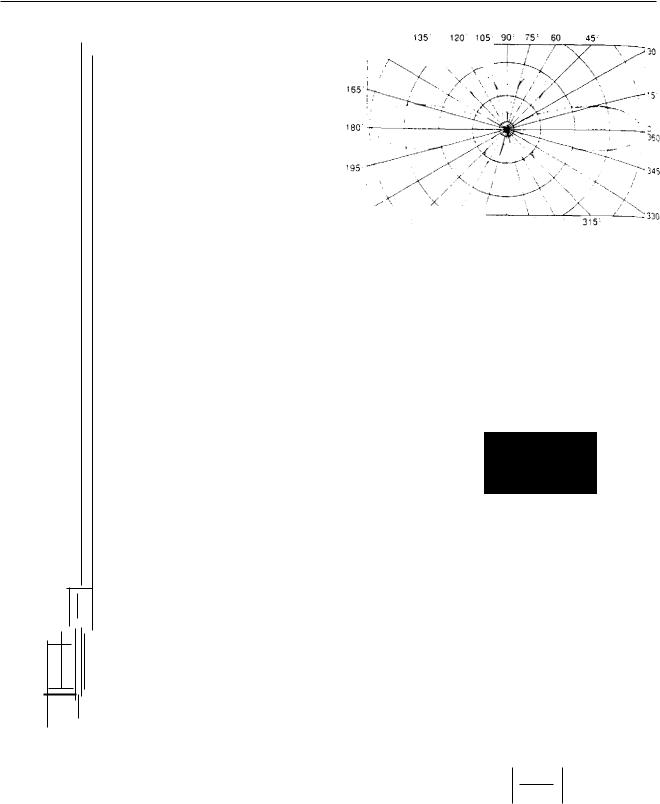
Figure 8.19 is the E-plane diagram for a Type CAT 80 antenna, which is the VHF low band version having a maximum gain of 3 dB with reference to a halfwave dipole. The graph circles therefore represent gains of 3 dB, 0 dB, —3 dB and —6 dB, starting at

GAIN 3db(VHF), 5db (UHF) -

SLIM, TAPERED DESIGN

RUGGED, GLASS-FIBRE PROTECTION:

FOAM ENCAPSULATION

EASY MOUNTING

FIG. 8.18 Philips Telecom VHF/UHF colinear antennas type CAT

the laigest reference circle and moving towards the centre.

Figure 8.20 is the 1-plane diagram for a Type CAT 460 antenna, which is the UHF version having a maximum gain of 5 dB with reference to a half-wave dipole. The graph circles therefore represent gains of 5 dB, 2 dB, —1 dB and 4 dB, starting at the largest reference circle.

The polar diagram shows a number of secondary lobes, the largest of which have gains of approximately

AM.

FIG. 8.19 E - plane polar diagram for a Philips VHF CAT 80 antenna

FIG. 8.20 E-plane polar diagram for a Philips UHF CAT 460 antenna

—2 dB with respect to a half-wave dipole in directions of 70 ° and 110 ° from the horizontal. The required bandwidth of the antenna will depend on the number of fixed station frequency channels which are to be transmitted or received and whether the antenna is to be used for transmit and receive functions. The bandwidth is conventionally taken as the frequency band between the 1.5 VSWR points on the VSWR/frequency graph for the antenna, where VSWR stands for the 'voltage standing wave ratio':

VSWR -=

Emin

where Em = voltage at crest of standing wave

E r„,,, = voltage at trough of standing wave

The VSWR is a measure of the impedance match between the characteristic impedance of the antenna

coaxial cable and the impedance of the antenna.

The characteristic impedance of a cable is the input impedance of an infinitely long length of the cable. In