reading / British practice / Vol D - 1990 (ocr) ELECTRICAL SYSTEM & EQUIPMENT

nology. The same applies for cables manufactured to CEGB Standards except that the values are not as widely available. The CEGB has its own computer program for this purpose which is used for instances where published data is not available. The source of the current ratings for power station cables are as follows:

In selecting this value it is assumed that drying out at the soil does not occur when the cable is carrying full-load current. This may not be the case in well

Jrained or loosely compacted soil, etc., for example, cand or made-up ground, and in these circumstances

a higher value must be used.

In this instance the external ihermal resistance consists of three parts, namely:

•The thermal resistance of the air space between the cable surface and the duet internal surface T4.

•The thermal resistance of the duct T.

•The external thermal resistance of the duct TZ.

Equations are available in IEC 287 for the calculation 01 each thermal resistance. The value of T4 is given b!, he sum of the individual thermal resistances, i.e.,

Values of thermal resistivity for the two duct materials ki , ed (taken from IEC 287) are given in Table 6.9.

TABLE 6.9

Values of thermal resistivity for duct installation

•Typical, as value varies with mix.

4.2.4Permissible current ratings

Tubulated ratings

there is no need to perform the calcula-

,tions. described to determine the current ratings for ahles manufactured to British Standards. This work

The current ratings for these cables are tabulated in Appendices C and D of this chapter for the three types of cable route described. As it is impractical to tabulate these for every possible variation under which the cables may be installed, these are presented for the set of standard installation conditions defined in the next . section. Rating factors are then given to enable the current rating to be corrected for any variation from these conditions. For convenience, the AC current ratings for two-core cables are also applied for DC operation.

If a circuit involves more than one type of cable route, e.g., a portion is laid in air and a portion buried direct in the ground, then the lowest of the current rating values (after application of any rating factors) must be used for the current rating of the cable. This is an important point when designing an external cable route as the decision on which type of cable route to use can make a difference to the size and hence cost of the cables required. For example, it can be seen from examination of the tables in Appendix D that for the larger sizes of multicore power cable the current rating is significantly reduced if laid in ducts, whereas if buried direct in the ground the current ratings are higher than in air for all except the largest cable size. With single-core power cables the reduction is of the same order, whether the cables are laid in ducts or buried direct in the ground.

Short lengths of duct (normally less than half a metre) are ignored for cable sizing purposes. The longitudinal conduction of heat by the cable metallic components is considered sufficient to maintain a uniform temperature rise.

Standard installation condition

The standard installation conditions for the tabulated current ratings are:

•Depth of duct (measured from the ground surface to the centre of the cable).

3.3 kV multicore power cables — 0.8 m.

•Duct thermal resistivity — 1.2 K.m/W,

•Method of installation

4.2.5 Rating factors

With conditions other than the standard installation conditions described, it is necessary to adjust the tabulated current rating to correct for the difference. This may be for a variation in the thermal parameters of the surrounding medium, i.e., ambient temperature, depth of burial or soil thermal resistivity, or because the cable is grouped with others.

The correction is performed by multiplying the tabulated current rating by a rating factor. The rating factor to be applied is obtained from tables produced for this purpose which cover the normal variations in installation conditions.

Where there is more than one variation to the standard installation conditions then the rating factor for each must be multiplied together to obtain the overall factor. Care is however required to ensure that only the relevant factors are applied to each section. For instance, if a portion of a cable route is in air and a portion buried in the ground, the rating factor for a different ambient air temperature is only applied to the laid in air current rating and that for a different depth of laying is only applied to the buried in the ground current rating, and not, as sometimes mistakenly happens, both applied throughout.

Rating factors for variations in thermal parameters

Tabulated rating factors are available for the following variations in the thermal parameters of the surroundings:

•Variation in ambient temperature (90 ° C and 70 ° C maximum conductor temperature).

•Variation in ground temperature (90 ° C and 70 ° C maximum conductor temperature) for cables laid direct in the ground.

Variation in depth of laying cables

•

ground.

Variation in soil thermal resistivity for cables laid

•direct in the ground.

•variation ,n soil thermal resistivity for cables laid in ducts.

•variation in depth of laying ducts.

wse rating factors are given in Appendix E of this

1.1

■ 11,1 pter.

Group rating factors

lt has earlier been mentioned that the current rating

for an isolated multicore cable or set of three singlecore cables needs to be reduced if installed in close

pro \imity to neighbouring cables. This is due to mutual

heating and applies irrespective of the type of cable

route. For cables laid

a %%all also has to be included. A reduction is avoided if cables are installed above certain minimum spacings

,thich, typically for cables laid in air, are shown in

Hg 6.19.

Unless the current rating is calculated for the method

of installation concerned, it follows that group rating must be applied to the isolated current ratings for

multicore cables or groups of three single-core cables

1k hen spaced apart by less than the minimum distance

necessary to achieve the isolated condition. This includes single - layer and multi - layer touching cables. The

typical rating factors for three spaced cables taken from ERA 69-30 Part III are shown in Fig 6.20.

Since the vast majority of power station cables are

laid in air it is highly desirable that adequate space is provided between these cables to allow the isolated current rating to be used. However this need has to be balanced against the cost of providing the additional

room and cable supporting steelwork to accommodate

551 5 De

O/ CF l'Yi0 CABLES

5)2 Oe

CW OF -D-rFEE CABLES

Power cable system design

the method of cable installation adopted derives benefit from avoiding any reduction due to group rating while at the same time efficiently utilises cable support steelwork space.

415 V. 3,3 kV and 11 kV single-core power cables

The method of installation is flat spaced in a singlelayer at 80 mm centres as shown in Fig 6.21. Ratings are calculated using this spacing.

apart by 25 mm as shown in Fig 6.22.

Where the two cables are of a different size, spacings are based on the larger of the two cable diameters to err on the safe side. On the same basis, if each cable size considered from the range of multicore cables is the cable with the highest number of cores, i.e., has the largest cable diameter, then all cables of this size with fewer cores are covered by this cable. Table 6.10 shows the axial spacings between these cables, using the cable design maximum overall diameters and the group rating factor. The lowest value of group rating Factor is 0.98 for the 3.3 kV 3-core 240 mm 2 and 415 V 4-core 300 mm 2 cables. Besides being almost negligible, if the argument on loading ratio made in the next section is applied, it is apparent that there is no need to apply group rating factors to these cables.

complex with heat also travelling outwards across adjacent cables and air pockets to reach the exterior surface of the cable group.

To determine the group rating factor, it is assumed that there is uniform heat generation throughout the cross-section of the cable group, from which it follows that the acceptable power loss from each cable is pro. portional to its cross-sectional area. Since the heat generation is uniform this also means that a cable can be located at any position within the group. On this basis, the group rating factor may be calculated if the heat dissipation coefficient and thermal resistivity of the group is known, i.e., the cable group is treated as behaving like a single cable. These parameters have been determined experimentally by the CEGB for a

(16 mm 2 and less) are random laid double-layer touching as shown in Fig

6.23.

RANDOM FILL

DOUBLE LAY5R

TOUCHING

FIG. 6.23 Method of installing multicore power cables (16 mm 2 and less)

through, but this cannot be used as a basis for calculating current ratings and the worst case must be assumed which is when the cables are tightly packed. In this situation, air flow between the cables is practically non-existent and heat dissipation is now more

double-layer group of cables, thus enabling the group rating factor for each cable size to be found.

At this point it is necessary to introduce the term loading ratio which is defined as the ratio of normal full-load current to permissible current rating after

applying any rating factor for variations in the thermal parameters. If a group rating factor is now applied to the permissible current rating, it follows that:

LR = IFL/Ip and OR

where LR = loading ratio

[FL = full load current

I p = permissible cable current after applying any rating factors for variations in thermal parameters

From the two equations it can be seen that provided LR OR there is no need to take account of the cable group rating factor.

Cables buried direct or in ducts

The same considerations as those just discussed can be applied to cables buried direct in the ground except that here the minimum spacings necessary to avoid a reduction in the current rating due to mutual heating are much greater. The net result is that group rating factors are applied where necessary. These are available from ERA 69-30 Part III for cables buried in flat formation with various axial spacings from touching to 0,6 m between cable centres for different numbers of cables in the group.

This situation is repeated for cables laid in ducts. Group rating factors are available for different spacings/formations of cable ducts for multicore and three single-core power cables.

FiG. 6.25 Cable installation with two and four cables per phase

This formation may be repeated for four cables per phase, by arranging the cable rows in tiers on separate steelwork levels as shown in the figure. Unfortunately this arrangement does not work with larger even numbers or odd numbers of cables per phase and the only way to achieve symmetry is by cable transposition. Transposition involves the interchange of cable positions so that each cable occupies the same space relative to the others for approximately onethird of the cable route length, as shown in Fig 6.26.

4.2.6 Single-core cables in parallel

Current sharing

Feeder circuits are frequently required to transfer high levels of power with currents up to 3000 A. Single -core cables are used for this purpose and from examination of the ratings for single-core cables, it can be seen that 1:1..eral cables in parallel per phase are needed.

With this arrangement, it is necessary to ensure that he current is shared approximately equally between each cable in parallel and that individual cables are not overloaded by exceeding their permissible current

rating. This is particularly important for cables laid )paced in flat formation where lack of symmetry, as

)hown in Fig 6.24 for two cables per phase, results in unequal current sharing.

Fig. 6.24 Lack of cable symmetry

I -

TOTAL LENGTH OF CABLE I

FIG. 6,26 Cable transposition

The CEGB has developed a computer program CURB03 [5] to calculate the current sharing between cables in parallel. To determine the current in each cable, the cable axial co-ordinates and length for each route section are entered into the computer program, together with the number of cables per phase, phase current, cable conductor resistance, armour details, etc. The output from the computer contains the current in

each cable which is checked against the cable permissible current rating as described earlier. The computer also calculates the voltage drop in the cables.

Sheath voltage

As mentioned in Section 4.2.3 of this chapter, the bonding of single-core power cables at one end only produces a standing voltage on the metallic screen/ armour. This voltage appears across the cable sheathing (hence is usually called the sheath voltage); its magnitude is proportional to the conductor current and cable route length, the maximum value appearing at the cable screen/armour insulated (open) end. At full load current, the standing voltage on the screen/ armour which is connected to the cable gland must not exceed the maximum allowable touch voltage of 55 V (see Section 11.2.2 of this chapter). In the event of a through fault, the induced voltage will reach a much higher value for the short duration of the fault. The cable oversheath and the gland insulation are designed to withstand this voltage up to a limit of 2 kV. To protect personnel from this condition, the accessible metal body of the cable gland is covered with a

PVC shroud. It is necessary to calculate the sheath voltage for these two conditions to ensure that the maximum voltages do not exceed the above limits. The two sheath voltage conditions described above are illustrated in Fig 6.27.

SINGLE CORE POWER CABLE

GLAND CONNECTION

TO EARTH

STANDING VOLTAGE UNDER

NORMAL OPERATION <555/

UP TO A MAXIMUM FOR

A THROUGH FAULT <2kV

Fin. 6.27 Sheath voltage

For cables installed in flat formation without transposition, the standing sheath voltage on the centre cable differs from that on the two outer cables. The sheath voltage for the centre cable is given by:

For most power cables ri = r2 =r, from which it can be shown that:

[2r - rf)] log, (r2/ri) =

Hence Vs = 47rfI 10 -7 log, (sir) V/m

The standing sheath voltage for the outer cables is given by:

Vs = j2.7rfI 10 11 - [2r /(ri - ri)] log, (r2/r 1 ) + 2 log, ('12s/r2) ± 1og 0 2) V/m again if r1 = r2 = r

Vs = j2irfl 10 -7 [2 loge (V2s/r) ± j-s/3 log e ] V/m then in magnitude

Vs1 = 27rfI 10 -7 ([2 log, (N/2 s/r)] 2

+ (V3 log, 2) 2 ) 2 Virn

27rfl 10 -7 42 Logi, (-12 s/r)I 2 + 1.44) 2 Vial

The standing sheath voltages with transposed cables are all equal and are given by:

V s = 27rfl 10 - 7 (1 - [2r/(ri - ri)1 log (r2/ri) + 2 log n (3-s/2s/r2)) V/m

again if r1 = r2 = r

Vs = 47rfl 10 -7 log, (3./2s/r2) V/m

The sheath voltage can also be calculated usir , he CEGB computer program CURB03. For practical purposes, the sheath voltage under short-circuit conditions can be taken as the full load current sheath voltage increased in proportion to the ratio of the short-circuit current to the full load current, as shown in the following expression:

VSC = VFL X ISC/IFL

where Vsc = short-circuit sheath voltage VFL = standing sheath voltage

Isc = short-circuit current

Vs -= 27rfI 10 -7 (1 - [2r/(1- 3 - r1)] log0(r2/rt) + 2 log 0 (s/r2)) V/m

where f = frequency, Hz

= full load current, A

r = inner radius of cable armour, m

r2 = outer radius of cable armour, m

s = separation between centres of adjacent cables, in

'FL = full load current

Design values for short circuit current are given in Table 6.11.

If the standing or short-circuit sheath voltage is found to exceed the maximum permitted, it becomes necessary to solid-bond the cable screen/armour at both ends and fit a sheath interrupter at the approxi-

mate mid-point of the cable route. A sheath interrupter is a device which allows the removal of a short length

4.3 Fault current and duration

The foregoing has described the process of determining the conductor size for a cable which will ensure that the maximum conductor temperature of the insulation is not exceeded during continuous operation. During a fault, however, abnormal currents can result in much higher temperatures which, unless the cable is adequately protected, could cause serious damage to the insulation or at worst start a cable fire. Insulation damage can occur over a period of several hours due to an overload, or within a fraction of a second due to a short-circuit or an earth fault. It is therefore equally important with power cable system design to ensure that the cable is adequately protected against all forms of excess current. This is achieved by coordinating the operating characteristics of the circuit protection with the fault current capability of the cable.

4.3.1 Short - circuit faults

I1 is appropriate to commence with a review of the c_ie n short-circuit current (due to a three-phase shortircuit) used at each system voltage level, as shown in Fable 6.11, and the types of fault current breaking device and main protection used for feeder and motor

ircuits, as shown in Appendix I. In this respect, feeder Nuits include interconnector and transformer circuits. The total clearance time for a fault cleared by a cIrcuit-breaker may be taken as the sum of the protection relay operating time and circuit-breaker open- ing ti me. With high set instantaneous overcurrent as

1 1 , 1 , „ nmE

FAULT CLEARED

FIG. 6.28 Oscillogram of current in one phase of a three-phase short-circuit

The same concern about failure to operate is not held about a fuse. Therefore, the total fault clearance time for fuse protected circuits is given by the maximum pre-arcing time, i.e., the energy let-through time determined from the fuse time versus current characteristic, of the circuit fuse. At 415 V, the largest size of fuse fitted is 800 A used on feeder circuits. Assuming maximum short-circuit current, the pre-arcing time with this fuse is about 0.01 s. This means that circuit interruption occurs during the first half cycle of the fault current.

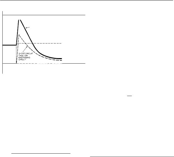
The sudden rush of current causes the conductor temperature to rise at an extreme race. Disconnection is followed by a period of fairly rapid cooling. The rise in conductor temperature is typically as shown in Fig 6.29, with the cable initially carrying rated current. The conductor is at the maximum conductor temperature and rises to a peak at the maximum short -circuit conductor temperature. If the cable had been initially

TEMP

MAXIMUM SHORT CIRCUIT CONDUCTOR TEMP

SHORT CMCLIIT FAULT DURING

NORMAL OPERA PON

YAMMUMCONDUCTORTEMP

AMBIENT TEMP

FIG. 6.29 Short-circuit conductor temperature rise

unloaded, the temperature rise from ambient would be as shown dotted.

As the duration of the temperature rise is short, the cable insulation and other components can withstand considerably higher temperatures without suffering permanent damage. By international agreement, standard maximum short-circuit conductor temperatures have been assigned to the commonly used cable materials. Several of these are given in Table 6.12.

TABLE 6.12

Maximum short-circuit conductor temperature

Two assumptions are made to assist with the calculation of the short-circuit temperature rise for circuitbreaker controlled circuits. The first is that all the heat energy produced is absorbed by the current carrying components, i.e., the temperature rise is adiabatic. The second is that over the duration of the short-circuit the current remains constant.

The effects of the current initial asymmetry and slight fall-off in current due to the increase in circuit resistance with temperature can be regarded as negligible. In practice, a certain amount of heat is absorbed

by the adjacent cable components and the error this introduces provides a margin of safety.

The temperature rise is calculated by equating the energy input to the energy absorbed expressed by the following formula:

1 2 t = K 2 S 2 log n [(Of + O )/(O; + i3)] where I = short-circuit current rms, A

=duration of short-circuit, s

K= constant depending on the material of the current carrying component

= reciprocal of temperature coefficient of resistance of current carrying component at 0° C

Qc (0 + 20)]T

where Qc = volumetric specific heat of the current carrying component at 20 ° C, J/°C mm 3

e2o = resistivity of current carrying component at 20° C, f2 mm

The constants for different conductor materials are given in Table 6.13.

TABLE 6.13

Material constants for fault calculations

It can be seen that since the temperature rise is adiabatic it is independent of the number of cable conductors. It should also be noted that when used for metallic screens, this formula indicates much higher temperatures than actually occur in practice and therefore must be used with some discretion.

For cable sizing purposes it is convenient to assume that the cable is operating at the maximum conductor temperature when the short-circuit occurs, and that the peak temperature reached is the maximum short-circuit conductor temperature. For a given cable insulation/ type, this leaves the short-circuit current, duration and cable sizes as variables and these may be plotted graphically (as shown in Fig 6.30) with initial and final

•20

0L0

FIG. 6.30 Short-circuit ratings of XLPE/EPR insulated cables with aluminium conductors

temperatures of 90 ° C and 250 ° C respectively, i.e., a 160 ° C temperature rise.

Using the above assumptions and the maximum short - circuit current, the minimum size cable required can also be calculated for a range of total fault clearance times. These are shown in Table 6.14 for single- core power cables at each system voltage.

With earth faults, both the conductor and the metallic screen/armour (which provide a low impedance path for earth fault current to return to the system neutral) need to be considered. Clearly, the temperature reached by each fault current-carrying component must not cause thermal damage to the cable. The maximum short-circuit temperature of the insulation and bedding must not be exceeded with fault current in the metallic screen and similarly the maximum short-circuit temperature of the bedding and oversheath must not be exceeded with fault current in the armour. Using the same expression for the adiabatic temperature rise and the material constants given in Table 6.13, the minimum cross-sectional area for the metallic screen/ armour can be calculated. In this instance:

I = earth fault current, A

t = duration of earth fault, s

S = area of metallic screen/armour, mm 2

I3f = final metallic screen/armour temperature, ° C

e t = initial temperature of the metallic screen/ armour, ° C

if it can be established that the cable will always be operating at a temperature less than the maximum conductor temperature, then the minimum cross-sec-

tional area may be calculated for the lower temperature concerned..

With circuits protected by

temperature is determined by the 1 2 1 'let-through energY' of the fuse. Fuse manufacturers provide 1 2 t values tor each fuse size from which the minimum cable crosswetional area can be calculated. This is not necessary With feeder circuits, as short-circuit requirements are automatically covered by the selection of a cable to match the fuse rating. However, this needs to be carried out for motor circuits as described in Section 4.6.2

The initial temperature for the metallic screen has to be calculated, but for the armour is taken as being 10 ° C below the maximum conductor temperature. The maximum temperature for the metallic screen/armour is normally the maximum short-circuit temperature for the sheathing material which, from Table 6.12, is 160° C. Cable armour cross-sectional areas are given in Appendix F of this chapter.

To determine the earth fault current it is necessary first to examine the method of system neutral earthing which, for a power station, is shown in Table 6.15.

At 3.3 kV and 11 kV the neutral earthing resistor limits the maximum earth fault current to 1000 A at each neutral: As two system supplies and hence two

INTERNAL

EARTH FAULT

ON ELITE PHASE

Flc. 6.31 Earth fault current path

It is considered that, in practice, earth fault currents are unlikely to exceed 2000 A and will probably be within the range 600-1000 A. For fuse protected circuits the clearance time for a given earth fault current can be determined from the fuse time versus current characteristic, enabling the armour temperature rise to be calculated. However, with aluminium armoured multicore cables to BS6346 it should be noted that the cross-sectional area of the armour wires is

•The current causing effective operation of the protective device (I2) does not exceed 1.45 times the lowest of the current carrying capacities (Iz) of any of the conductors of the circuit.

This may be summarised as:

In --C. IZ

12 1.45 lz

The circuit protection must operate with an overload up to 45 07o of rated current within a period accepted as being no more than 4 hours. While this more than doubles the conductor temperature rise, within this ti mescale, experience has shown that this does not result in unacceptable cable damage.

The overload protection of plant items such as motors or transformers is provided by IDMT or thermal overload relays. With the protection set correctly, the characteristics of these devices meet this overload criteria. As the overload capability of the cable is normally greater than that of the plant item, this arrangement automatically affords overload protection to the cable. The protection of 415 V feeder circuits with fuses to BS88: Part 2 [8] also meets this cable overload criteria.

Operation of the overload protection at not more than 1.45 times the current rating of the cable also applies to cables laid in ducts. With cables buried direct in the ground, the same rise in conductor temperature is reached with a smaller overload and therefore the maximum current at which the protection is designed