

2556 |
CHAPTER 31. BASIC PROCESS CONTROL STRATEGIES |
31.6.3Lead/Lag and dead time function blocks
The addition of dynamic compensation in a feedforward control system may require a lag function, a lead function, and/or a dead time function, depending on the nature of the time delay di erences between the relevant process load and the system’s corrective action. Modern control systems provide all these functions as digital function blocks. In the past, these functions could only be implemented in the form of individual instruments with these time characteristics, called relays. As we have already seen, lead and lag functions may be rather easily implemented as simple RC filter circuits. Pneumatic equivalents also exist, which were the only practical solution in the days of pneumatic transmitters and controllers. Dead time is notoriously di cult to emulate using analog components of any kind, and so it was common to use lag-time elements (sometimes more than one connected in series) to provide an approximation of dead time.
With digital computer technology, all these dynamic compensation functions are easy to implement and readily available in a control system. Some single-loop controllers even have these capabilities programmed within, ready to use when needed.
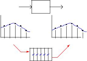
A dead time function block is most easily implemented using the concept of a first-in, first-out shift register, sometimes called a FIFO. With this concept, successive values of the input variable are stored in a series of registers (memory), their progression to the output delayed by a certain amount of time:
Input |
Dead |
Output |
|
time |
|||
|
|
t1 |
t2 |
t3 |
t4 |
t5 |
t0 |
t1 |
t2 |
t3 |
t4 |
t5 |
Shift register
t5 t4 t3 t2 t1
t5 t4 t3 t2 t1 t0
31.6. FEEDFORWARD WITH DYNAMIC COMPENSATION |
2557 |
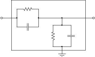
Lead and lag functions are also implemented digitally in modern controllers and control systems, but they are actually easier to comprehend in their analog (RC circuit) forms. The most common way lead and lag functions are found in modern control systems is in combination as the so-called lead/lag function, merging both lead and lag characteristics in a single function block (or relay):
|
R1 |
|
Vin |
Lead |
Vout |
C1 |
||
|
||
|
|
Lag |
|
R2 |
C2 |
Each parallel RC subcircuit represents a time constant (τ ), one for lead and one for lag. The overall behavior of the network is determined by the relative magnitudes of these two time constants. Which ever time constant is larger, determines the overall characteristic of the network.
2558 |
CHAPTER 31. BASIC PROCESS CONTROL STRATEGIES |
If the two time constant values are equal to each other (τlead = τlag ), then the circuit performs no dynamic compensation at all, simply passing the input signal to the output with no change except
for some attenuation:
|
|
|
R1 |
|
|
|
|
|
|
|
|
|
|
|
|
|
||
Vin |
|
Lead |
|
|
|
|
|
|
|
|
|
|
|
Vout |
||||
|
|
C1 |
|
|
|
|
|
|
|
|
|
|
|
|||||
|
|
|
|
|
|
|
|
|
|
|
|
|
||||||
|
|
|
|
|
|
|
|
|
|
|
|
|
|
|
|
|
||
|
|
|
|
|
|
|
|
|
|
|
|
|
|
|
|
|
|
|
|
|
|
|
|
|
|
|
|
Lag |
|
|
|
||||||
|
|
|
|
|
|
|
|
|
|
|
|
|||||||
|
R1C1 = R2C2 R2 |
|
|
C2 |
||||||||||||||
|
|
|
||||||||||||||||
|
|
|
|
|
|
|
|
|
|
|||||||||
|
|
|
|
|
|
|
|
|
|
|||||||||
|
|
|
|
|
|
|
|
|
|
|||||||||
|
τlead = τlag |
|
|
|
|
|
|
|
|
|
|
|
||||||
|
|
|
|
|
|
|
|
|
|
|
|
|
|
|
|
|
|
|
|
|
|
|
|
|
|
|
|
|
|
|
|
|
|
|
|
|
|
Vin
Vout
Time
Vin
Vout
Time
A square wave signal entering this network will exit the network as a square wave. If the input signal is sinusoidal, the output will also be sinusoidal and in-phase with the input.
31.6. FEEDFORWARD WITH DYNAMIC COMPENSATION |
2559 |
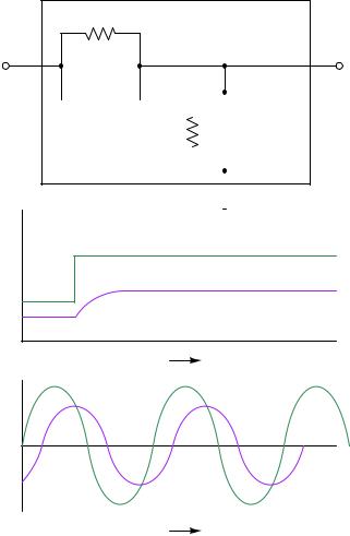
If the lag time constant exceeds the lead time constant (τlag > τlead), then the overall behavior of the circuit will be to introduce a first-order lag to the voltage signal:
|
R1 |
Lag-dominant |
Vin |
Lead |
Vout |
C1 |
||
|
|
|
|
|
|
|
|
|
|
|
|
|
|
|
|
|
|
|
|
|
|
Lag |
|
|
||||||
|
|
|
|
|
|
|
|
|||||||
R2C2 > R1C1 R2 |
|
|
C2 |
|||||||||||
|
|
|||||||||||||
|
|
|
|
|
|
|
|
|
||||||
|
|
|
|
|
|
|
|
|
||||||
|
|
|
|
|
|
|
|
|
||||||
τlag > τlead |
|
|
|
|
|
|
|
|
|
|
||||
|
|
|
|
|
|
|
|
|
|
|
|
|
|
|
|
|
|
|
|
|
|
|
|
|
|
|
|
|
|
Vin
Vout
Time
Vin
Vout
Time
A square wave signal entering the network will exit the network as a sawtooth-shaped wave. A sinusoidal input will emerge sinusoidal, but with a lagging phase shift. This, in fact, is where the lag function gets its name: from the negative (“lagging”) phase shift it imparts to a sinusoidal input.
2560 |
CHAPTER 31. BASIC PROCESS CONTROL STRATEGIES |
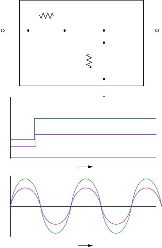
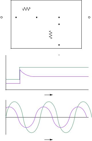
Conversely, if the lead time constant exceeds the lag time constant (τlead > τlag ), then the overall behavior of the circuit will be to introduce a first-order lead to the voltage signal (a step-change
voltage input will cause the output to “spike” and then settle to a steady-state value):
R1 Lead-dominant
|
|
|
|
|
|
|
|
|
|
|
|
|
|
|
|
|
|
|
Vin |
|
Lead |
|
|
|
|
|
|
|
|
|
|
|
Vout |
||||
|
|
C1 |
|
|
|
|
|
|
|
|
|
|
|
|||||
|
|
|
|
|
|
|
|
|
|
|
|
|
|
|
|
|
||
|
|
|
|
|
|
|
|
|
|
|
|
|
|
|
|
|
|
|
|
|
|
|
|
|
|
|
|
Lag |
|
|
|
||||||
|
|
|
|
|
|
|
|
|
|
|
|
|||||||
|
R1C1 > R2C2 R2 |
|
|
C2 |
||||||||||||||
|
|
|
||||||||||||||||
|
|
|
|
|
|
|
|
|
|
|||||||||
|
|
|
|
|
|
|
|
|
|
|||||||||
|
|
|
|
|
|
|
|
|
|
|||||||||
|
τlead > τlag |
|
|
|
|
|
|
|
|
|
|
|
||||||
|
|
|
|
|
|
|
|
|
|
|
|
|
|
|
|
|
|
|
|
|
|
|
|
|
|
|
|
|
|
|
|
|
|
|
|
|
|
Vin
Vout
Time
Vin
Vout
Time
A square wave signal entering the network will exit the network with sharp transients on each leading edge. A sinusoidal input will emerge sinusoidal, but with a leading phase shift. Not surprisingly, this is where the lead function gets its name: from the positive (“leading”) phase shift it imparts to a sinusoidal input.
31.6. FEEDFORWARD WITH DYNAMIC COMPENSATION |
2561 |
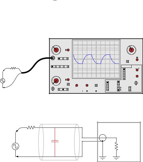
This exact form of lead/lag circuit finds application in a context far removed from process control: compensation for coaxial cable capacitance in a ×10 oscilloscope probe. Such probes are used to extend the voltage measurement range of standard oscilloscopes, and/or to increase the impedance of the instrument for minimal loading e ect on sensitive electronic circuits. Using a ×10 probe, an oscilloscope will display a waveform that is 101 the amplitude of the actual signal, and present ten times the normal impedance to the circuit under test.
If a 9 MΩ resistor is connected in series with a standard oscilloscope input (having an input impedance of 1 MΩ) to create a 10:1 voltage division ratio, problems will result from the cable capacitance connecting the probe to the oscilloscope input. What should display as a square-wave input instead looks “rounded” by the e ect of capacitance in the coaxial cable and at the oscilloscope input:
|
|
Volts/Div A |
|
|
|
|
|
Sec/Div |
|||
|
|
|
|
|
|
|
|
|
|
250 μ |
|
|
|
0.5 |
0.2 |
0.1 |
|
|
|
|
|
1 m |
50 μ |
|
|
1 |
|
50 m |
Position |
|
|
|
|
5 m |
10 μ |
|
|
2 |
|
20 m |
|
|
|
|
25 m |
2.5 μ |
|
|
|
5 |
|
10 m |
|
|
|
|
|
100 m |
0.5 μ |
|
|
10 |
|
5 m |
|
|
|
|
|
500 m |
0.1 μ |
|
|
20 |
|
2 m |
|
|
|
|
|
1 |
0.025 μ |
|
|
|
|
DC Gnd AC |
|
|
|
|
2.5 |
off |
|
|
|
|
|
|
|
|
|
|
|
||
|
|
|
|
|
|
|
|
|
|
X-Y |
|
|
9 MΩ |
A |
B |
Alt Chop Add |
|
|
|
|
|
Position |
|
|
|
|
|
|
Triggering |
|
|||||
|
|
|
|
|
|
|
|
|
|
Level |
|
|
|
|
|
|
|
|
|
|
|
A |
|
|
|
Volts/Div B |
|
|
|
|
|
B |
Holdoff |
||
|
|
|
|
|
|
|
Alt |
||||
|
|
0.5 |
0.2 |
0.1 |
|
|
|
|
|
Line |
|
|
|
1 |
|
50 m |
Position |
|
|
|
|
|
|
|
|
|
|
|
|
|
Ext. |
|
|||
Square wave |
|
2 |
|
20 m |
|
|
|
|
|
||
|
|
|
|
|
|
|
Ext. input |
||||
|
5 |
|
10 m |
|
|
|
|
|
|
||
generator |
|
|
Invert |
Intensity |
Focus |
Beam find |
Norm |
AC |
|
||
|
10 |
|
5 m |
|
|||||||
|
|
20 |
|
2 m |
|
|
|
|
Auto |
DC |
|
|
|
|
|
DC Gnd AC |
Off |
|
|
Single |
Slope |
LF Rej |
|
|
|
|
|
|
|
|
|
Reset |
|||
|
|
|
|
|
|
Cal 1 V Gnd |
Trace rot. |
HF Rej |
|||
|
|
|
|
|
|
|
|||||
The reason for this is signal distortion the combined e ect of the 9 MΩ resistor and the cable’s natural capacitance forming an RC network:
|
9 MΩ |
Coaxial probe cable |
Oscilloscope |
|
|
|
|
||
|
|
|
|
|
|
|
|
BNC connector |
|
Square wave |
|
Ccable |
R |
scope |
generator |
|
|
1 MΩ |
|
2562 |
CHAPTER 31. BASIC PROCESS CONTROL STRATEGIES |
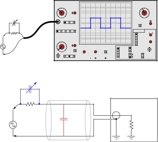
A simple solution to this problem is to build the 10:1 probe with a variable capacitor connected in parallel across the 9 MΩ resistor. The combination of the 9 MΩ resistor and this capacitor creates a lead network to cancel out the e ects of the lag caused by the cable capacitance and 1 MΩ oscilloscope impedance in parallel. When the capacitor is properly adjusted, the oscilloscope will accurately show the shape of any waveform at the probe tip, including square waves:
|
Volts/Div A |
|
|
|
|
|
Sec/Div |
|||
|
|
|
|
|
|
|
|
|
250 μ |
|
|
0.5 |
0.2 |
0.1 |
|
|
|
|
|
1 m |
50 μ |
|
1 |
|
50 m |
Position |
|
|
|
|
5 m |
10 μ |
|
2 |
|
20 m |
|
|
|
|
25 m |
2.5 μ |
|
|
5 |
|
10 m |
|
|
|
|
|
100 m |
0.5 μ |
Compensated probe |
10 |
|
5 m |
|
|
|
|
|
500 m |
0.1 μ |
20 |
|
2 m |
|
|
|
|
|
1 |
0.025 μ |
|
|
|
|
DC Gnd AC |
|
|
|
|
2.5 |
off |
|
|
|
|
|
|
|
|
|
|
||
|
|
|
|
|
|
|
|
|
X-Y |
|
9 MΩ |
A |
B |
Alt Chop Add |
|
|
|
|
|
Position |
|
|
|
|
|
Triggering |
|
|||||
|
|
|
|
|
|
|||||
|
|
|
|
|
|
|
|
|
Level |
|
|
|
|
|
|
|
|
|
|
A |
|
|
Volts/Div B |
|
|
|
|
|
B |
Holdoff |
||
|
|
|
|
|
|
Alt |
||||
|
0.5 |
0.2 |
0.1 |
|
|
|
|
|
Line |
|
|
1 |
|
50 m |
Position |
|
|
|
|
|
|
|
|
|
|
|
|
Ext. |
|
|||
Square wave |
2 |
|
20 m |
|
|
|
|
|
||
|
|
|
|
|
|
Ext. input |
||||
5 |
|
10 m |
|
|
|
|
|
|
||
generator |
|
Invert |
Intensity |
Focus |
Beam find |
Norm |
AC |
|
||
10 |
|
5 m |
|
|||||||
|
|
|
|
|
|
|
|
|
||
|
20 |
|
2 m |
|
|
|
|
Auto |
DC |
|
|
|
|
DC Gnd AC |
Off |
|
|
Single |
Slope |
LF Rej |
|
|
|
|
|
|
|
|
Reset |
|||
|
|
|
|
|
Cal 1 V Gnd |
Trace rot. |
HF Rej |
|||
|
|
|
|
|
|
|||||
Ccompensation
|
9 MΩ |
Coaxial probe cable |
Oscilloscope |
|
|
|
|
||
|
|
|
|
|
|
|
|
BNC connector |
|
Square wave |
|
Ccable |
R |
scope |
generator |
|
|
1 MΩ |
|
31.6. FEEDFORWARD WITH DYNAMIC COMPENSATION |
2563 |
If we re-draw this compensated probe circuit to show the resistor pair and the capacitor pair both working as 10:1 voltage dividers, it becomes clearer to see how the two divider circuits work in parallel with each other to provide the same 10:1 division ratio only if the component ratios are properly proportioned:
Vinput
(probe tip)
|
|
|
|
|
|
|
|
|
|
|
|
Compensation is effective because |
9 R |
|
|
|
|
|
|
|
|
|
C |
(9R)(C) = (R)(9C) |
|
|
|
|
|
|
|
|
|
|
||||
(Rprobe) |
|
|
|
|
|
|
|
|
|
(Ccompensation) |
τ1 = τ2 |
|
|
|
|
|
|
|
|
|
|
Vscope |
|||
|
|
|
|
|
|
|
|
|
|
|
|
|
R |
|
|
|
|
|
|
|
|
|
9 C |
||
|
|
|
|
|
|
|
|
|
|
|||
|
|
|
|
|
|
|
|
|
|
|||
(Rscope) |
|
|
|
|
|
|
|
|
|
(Ccable) |
|
|
|
|
|||||||||||
|
|
|
|
|
|
|
|
|
|
|
|
|
|
|
|
|
|
|
|
|
|
|
|
|
|
|
|
|
|
|
|
|
|
|
|
|
|
|
The series resistor pair forms an obvious 10:1 division ratio, with the smaller of the two resistors being in parallel with the oscilloscope input. The upper resistor, being 9 times larger in resistance value, drops 90% of the voltage applied to the probe tip. The series capacitor pair forms a less obvious 10:1 division ratio, with the cable capacitance being the larger of the two. Recall that the reactance of a capacitor to an AC voltage signal is inversely related to capacitance: a larger capacitor will have fewer ohms of reactance for any given frequency according to the formula XC = . Thus, the capacitive voltage divider network has the same 10:1 division ratio as the resistive voltage divider network, even though the capacitance ratios may look “backward” at first glance.
2564 |
CHAPTER 31. BASIC PROCESS CONTROL STRATEGIES |
If the compensation capacitor is adjusted to an excessive value, the probe will overcompensate for lag (too much lead), resulting in a “spiked” waveform on the oscilloscope display with a perfect square-wave input:
|
Volts/Div A |
|
|
|
|
|
Sec/Div |
|||
|
|
|
|
|
|
|
|
|
250 μ |
|
|
0.5 |
0.2 |
0.1 |
|
|
|
|
|
1 m |
50 μ |
Consequence of an |
1 |
|
50 m |
Position |
|
|
|
|
5 m |
10 μ |
2 |
|
20 m |
|
|
|
|
25 m |
2.5 μ |
||
overcompensated probe |
5 |
|
10 m |
|
|
|
|
|
100 m |
0.5 μ |
|
10 |
|
5 m |
|
|
|
|
|
500 m |
0.1 μ |
|
20 |
|
2 m |
|
|
|
|
|
1 |
0.025 μ |
|
|
|
DC Gnd AC |
|
|
|
|
2.5 |
off |
|
|
|
|
|
|
|
|
|
|
||
|
|
|
|
|
|
|
|
|
X-Y |
|
9 MΩ |
A |
B |
Alt Chop Add |
|
|
|
|
|
Position |
|
|
|
|
|
Triggering |
|
|||||
|
|
|
|
|
|
|||||
|
|
|
|
|
|
|
|
|
Level |
|
|
|
|
|
|
|
|
|
|
A |
|
|
Volts/Div B |
|
|
|
|
|
B |
Holdoff |
||
|
|
|
|
|
|
Alt |
||||
|
0.5 |
0.2 |
0.1 |
|
|
|
|
|
Line |
|
|
1 |
|
50 m |
Position |
|
|
|
|
|
|
|
|
|
|
|
|
Ext. |
|
|||
Square wave |
2 |
|
20 m |
|
|
|
|
|
||
|
|
|
|
|
|
Ext. input |
||||
5 |
|
10 m |
|
|
|
|
|
|
||
generator |
|
Invert |
Intensity |
Focus |
Beam find |
Norm |
AC |
|
||
10 |
|
5 m |
|
|||||||
|
|
|
|
|
|
|
|
|
||
|
20 |
|
2 m |
|
|
|
|
Auto |
DC |
|
|
|
|
DC Gnd AC |
Off |
|
|
Single |
Slope |
LF Rej |
|
|
|
|
|
|
|
|
Reset |
|||
|
|
|
|
|
Cal 1 V Gnd |
Trace rot. |
HF Rej |
|||
|
|
|
|
|
|
|||||
With the probe’s compensating capacitor exhibiting an excessive amount of capacitance, the capacitive voltage divider network has a voltage division ratio less than 10:1. This is why the waveform “spikes” on the leading edges: the capacitive divider dominates the network’s response in the short term, producing a voltage pulse at the oscilloscope input greater than it should be (divided by some ratio less than 10). Soon after the leading edge of the square wave passes, the capacitors’ e ects will wane, leaving the resistors to establish the voltage division ratio on their own. Since the two resistors have the proper 10:1 ratio, this causes the oscilloscope’s signal to “settle” to its proper value over time. Thus, the waveform “spikes” too far at each leading edge and then decays to its proper amplitude over time.
While undesirable in the context of oscilloscope probes, this is precisely the e ect we desire in a process control lead function. The purpose of a lead/lag function is to provide a signal gain that begins at some initial value, then “settles” at another value over time. This way, sudden changes in the feedforward signal will either be amplified or attenuated for a short duration to compensate for lags in other parts of the control system, while the steady-state gain of the feedforward loop remains at some other value necessary for long-term stability. For a lag function, the initial gain is less than the final gain; for a lead function, the initial gain exceeds the final gain. If the lead and lag time constants are set equal to each other, the initial and final gains will likewise be equal, with the function exhibiting a constant gain at all times.

31.6. FEEDFORWARD WITH DYNAMIC COMPENSATION |
2565 |
Although lead-lag functions for process control systems may be constructed from analog electronic components, modern systems implement the function arithmetically using digital microprocessors. A typical time-domain equation describing a digital lead/lag function block’s output response (y) to an input step-change from zero (0) to magnitude x over time (t) is as follows:
!
τlead − τlag
y = x 1 + t
τlag e τlag
As you can see, if the two time constants are set equal to each other (τlead = τlag ), the second term inside the parentheses will have a value of zero at all times, reducing the equation to y = x.
If the lead time constant exceeds the lag time constant (τlead > τlag ), then the fraction will begin with a positive value and decay to zero over time, giving us the “spike” response we expect from a
lead function. Conversely, if the lag time constant exceeds the lead (τlag > τlead), the fraction will begin with a negative value at time = 0 (the beginning of the step-change) and decay to zero over time, giving us the “sawtooth” response we expect from a lag function.
It should also be evident from an examination of this equation that the “decay” time of the lead/lag function is set by the lag time constant (τlag ). Even if we just need the function to produce a “lead” response, we must still properly set τlag in order for the lead response to decay at the correct rate for our control system. The intensity of the lead function (i.e. how far it “spikes” when
presented with a step-change in input signal) varies with the ratio τlead , but the duration of the
τlag
“settling” following that step-change is entirely set by τlag .
2566 |
CHAPTER 31. BASIC PROCESS CONTROL STRATEGIES |
To summarize the behavior of a lead/lag function:
•If τlead = τlag , the lead/lag function will simply pass the input signal through to the output (no lead or lag action at all)
•If τlead = 0, the lead/lag function will provide a pure lag response with a final gain of unity and a time constant of τlag
•If τlead = 2(τlag ), the lead/lag function will provide a lead response with an initial gain of 2, a final gain of unity, and a time constant of τlag
τlead = 0 |
In |
|
|
|
|
|
|
|
|
|
Out |
|
|
|
|||
|
|
Time |
|
|
|
|
|
|
|
|
|
|
|
||||
|
|
|
|
|
|
|
|
|
|
|
|
|
|
|
|
||
τlead = 1/2 τlag |
In |
|
|
|
|
|
|
|
|
|
Out |
|
|
|
|||
|
|
|
|
|||||
|
|
|
|
|
|
|
|
|
|
|
Time |
|
|
|
|
||
|
|
|
|
|
||||
|
|
|
|
|
|
|
|
|
|
|
|
|
|
|
|
|
|
τlead = τlag |
|
|
|
|
|
|
|
|
In |
|
|
Out |
|
|
|||
|
|
Time |
|
|
|
|
|
|
|
|
|
|
|
||||
|
|
|
|
|
|
|
||
|
|
|
|
|
|
|||
τlead = 3/2 τlag |
In |
|
Out |
|
|
|||
|
|
|
||||||
|
|
|
|
|
|
|
||
|
|
|
|
|
|
|
||
|
|
|
|
|
|
|
|
|
|
|
|
|
|
|
|||
|
|
Time |
|
|
|
|
||
|
|
|
|
|
||||
|
|
|
|
|
|
|||
|
|
|
|
|
|
|
|
|
τlead = 2τlag |
In |
|
Out |
|
|
|||
|
|
|
||||||
|
|
|
|
|
|
|
||
|
|
|
|
|
|
|
||
|
|
|
|
|
|
|
|
|
|
|
|
|
|
|
|||
|
|
Time |
|
|
|
|
||
|
|
|
|
|
||||
|
|
|
|
|
|
|
|
|