акустика / gan_ws_acoustical_imaging_techniques_and_applications_for_en

interpolated continuous image from the sampled image if the x, y sampling frequencies are greater than twice the bandwidths, that is, if

Equivalently, if the sampling intervals are smaller than one-half of the reciprocal of bandwidths, that is, if

11

then F(ξ1, ξ2 )can be recovered by a low-pass filter with frequency response

0, otherwise

where R is any region whose boundary ∂R is contained within the annular ring between the rectangles R1 and R2.

3.3.3Nyquist Rate

The lower bounds on the sampling rate in (3.46) are called the Nyquist rates or the Nyquist frequencies. Their reciprocals are called the Nyquist intervals. The sampling theory states that a band-limited image sampled above its x and y Nyquist rates can be recovered without error by low-pass filtering the sampled image. However, if the sampling frequencies are below the Nyquist frequency, that is, if ξxs < 2ξx0, ξys < 2ξy0, then the periodic replications of F (ξ1, ξ2 ) will overlap, resulting in a distorted spectrum Fs (ξ1, ξ2 ) from which F (ξ1, ξ2 ) is irrevocably lost.

3.3.4Sampling Theorem

A band-limited image f (x, y) satisfying (3.45) and sampled uniformly on a rectangular grid with spacing x, y, can be recovered without error from the sample values f (m x, n y) provided the sampling rate is greater than the Nyquist rate, that is, 1x = ξxs > 2ξx0, 1y =

ξyx > 2ξy0

3.3.5Examples of Application of Two-Dimensional Sampling Theory

A common example is a sampling theory for the random noise that is always present in the image. Here, we have to deal with random fields. A continuous stationary random field f (x, y) is called band-limited if its power spectral density function (SDF) S(ξ1, ξ2 ) is band-limited, that is, if S(ξ1, ξ2 ) = 0 for |ξ 1| > ξ x0 and |ξ 2| > ξ y0.

3.3.6Sampling Theorem for Radom Fields

If f (x, y) is a stationary band-limited random field, then

This theorem states that if the random field f (x, y) is sampled above its Nyquist rate, then a continuous random field f¯(x, y) can be reconstructed from the sampled sequences such that f¯(x, y) converges to f in the mean-square sense.

3.3.7Practical Limitation in Sampling and Reconstruction

The above sampling theory is based on several idealizations. Real-world images are not band-limited, which means that aliasing errors can occur. These can be reduced by filtering the input image prior to sampling, but at the cost of attenuating higher spatial frequencies. Such a loss in resolution, which results in a blurring of the image, also occurs because practical scanners have finite apertures. Finally, the reconstruction system can never be the ideal low-pass filter required by the sampling theory as its transfer function depends on the display aperture.

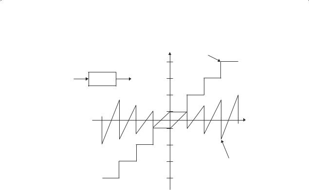
3.3.8Image Quantization

The second step in image digitization is quantization. A quantizer maps a continuous variable u into a discrete variable u , which takes values from a finite set {r1, r2, . . . . . . .rt } of numbers. This mapping is generally a staircase function and the quantization rule is as follows: Define {tk, k = 1, . . . . . . . . . L + 1} as a set of increasing transition or decision levels with t1 and tL+1

3.4Stochastic Modelling of Images

In image processing works, there are a number of random variables to be involved. As statistics is frequently used to deal with random data, we will also use stochastic models to represent images. The terms used in statistics, such as means and covariance functions, will also be used here.

Figure 3.5 A quantizer (Jain [2])

We start with a one-dimensional (1D) linear system to represent the input signals. Examples of stochastic models used here are covariance models, 1D autoregressive (AR) models, 1D moving average (MA) models, and 1D autoregressive moving average (ARMA) models.

3.4.1Autoregressive Models

Let u(n) be a real, stationary random sequence with zero mean and covariance r(n). Let ε(n) be the input and H(z) the transfer function of the linear system, then the SDF of u(n) is given by

n=0

and all its poles lie inside the unit circle [3].

A zero mean random sequence u(n) is called an AR process of order P when it can be generated as the output of the system.

The system used the most recent P outputs and the current input to generate the next output recursively.

3.4.2 Properties of AR Models

The quantity

k=1

is the best linear mean square predictor of u(n) based on all its past, but it depends only on the previous P samples. For Gaussian sequences this means that a pth-order AR sequence is a Markov-P process.

3.4.3Moving Average Model

A random sequence u(n) is called a MA process of order q when it can be written as a weighted running average of uncorrelated random variables

k=0

where ε(n) is a zero mean white noise process of variance β2. The SDF of this MA is given by

k=0

3.5Beamforming

Beamforming is a signal processing technique used in sensor arrays for directional signal transmission or reception. Beamforming can be used for sound waves or radio waves, but here we will focus only on sound waves as it has numerous applications in sonar, speech, and siesmology. The spatial selectivity is achieved by using adaptive or fixed receive/transmit beam patterns. The improvement compared with an omnidirectional reception/transmission is known as the receive/transmit gain (or loss).

3.5.1Principles of Beamforming

The principle is briefly shown in Figure 3.6. Beamforming takes advantage of interference to change the directionality of the array. When transmitting, a beamformer controls the phase and relative amplitude of the signal at each transmitter, in order to create a pattern of constructive and destructive interference in the wavefront. When receiving, the information from

UL Transmission: sounding signal

Ch

Est

Desired user

MS

B/F

DL Tx

Interfering user

MS

Figure 3.6 Principle of beamforming (Wikipedia [4])

different sensors is combined in such a way that the expected pattern of radiation is preferentially observed.

Sending a sharp pulse of underwater sound towards a ship in the distance by simply transmitting a sharp pulse from every sonar projector in an array simultaneously, leads to failure because the ship will first hear the pulse from the speaker that happens to be nearest, and later pulses form speakers that happen to be further from the ship. The beamforming technique involves sending the pulse from each projector at slightly different times (the projector closest to the ship being last) so that every pulse hits the ship at exactly the same time, producing the effect of a single strong pulse from a single powerful projector. The same principle can also be carried out in air using loudspeakers.

In passive sonar, and in reception in active sonar, the beamforming technique involves combining delayed signals from each hydrophone at slightly different times. The hydrophones closest to the target will be combined after the longest delay, so that every signal reaches the output at exactly the same time, making one loud signal that seemed to come from a single, very sensitive hydrophone. Receive beamforming can also be used with microphones.

Beamforming techniques can be divided into two categories:

1.Conventional beamformers: fixed or switched beam mode.

2.Adaptive beamformers or adaptive arrays: desired signal maximization mode; or interference signal minimization or cancellation mode.

Conventional beamformers use a fixed set of weightings and time-delays (or phasings) to combine the signals from the sensors in the array, primarily using only information about the location of the sensors in space and the wave directions of interest. In contrast, adaptive beamforming techniques generally combine this information with properties of the signals actually received by the array, typically to improve rejection of unwanted signals from other directions. This process may be carried out in either the time or the frequency domain.

As the name suggests, the adaptive beamformer is able to automatically adapt its response to different situations, although some criterion has to be set up to allow the adaption to proceed, such as minimizing the total noise output. Owing to the variation of noise with frequency, it may be desirable in wide-band systems to carry out the process in the frequency domain.

Beamforming can be computationally intensive. A sonar-phased array has a data rate that is low enough to allow it to be processed in real-time in software that is flexible enough to transmit and/or receive in several directions at once.

3.5.2Sonar Beamforming Requirements

Sonars have many applications, such as wide-area search-and-ranging, and underwater imaging such as the side-scan sonar and acoustic cameras.

Sonar applications vary from 1 Hz to 2 MHz and array elements may be few and large, or number in the hundreds yet be very small. This will shift beamforming design efforts significantly between the system’s upstream components (transducers, preamps and digitizers) and the actual downstream beamformer computational hardware. High-frequency, focused beam, multielement imaging search sonars and acoustic cameras often require fifth-order spatial processing.

Many sonar systems, such as on torpedoes, consist of arrays of possibly 100 elements that must accomplish beamsteering over a 100-degree field of view and work in both active and passive modes. Sonar arrays are used both actively and passively in one, two and three dimensions:

One-dimensional line arrays are usually in multielement passive systems towed behind ships and in a single or multielement side-scan sonar.

Two-dimensional planar arrays are common in active/passive ship hull-mounted sonars and some side-scan sonars.

Three-dimensional spherical and cylindrical arrays are used in sonar domes in modern submarines and ships.

Sonar differs from radar. In some applications, such as wide-area-search, all directions often need to be listened to, and broadcast to, simultaneously, thus requiring a multibeam system. In a narrowband sonar receiver the phases for each beam can be manipulated entirely by signal processing software, as compared to current radar systems that use hardware to listen in a single direction at a time.

Sonar also uses beamforming to compensate for the significant problem of the slower propagation speed of sound compared to that of electromagnetic radiation. In side-look sonars, the speed of the towing system, or vehicle carrying the sonar, is sufficient to move the sonar out of the field of returning sound. In addition to focusing algorithms intended to improve reception, many side-scan sonars also employ beamsteering to look forward and backward to capture incoming pulses that would have been missed by a single side-looking beam.

3.6Finite-Element Method

3.6.1Introduction

The finite-element method (FEM) originated from the need to solving complex elasticity and structural problems in civil and aeronautical engineering. Its development can be traced back to the work of Alexander Hrennikoff (1941) and Richard Courant (1942) [3]. While the approaches used by these pioneers are different, they shared one essential characteristic: mesh

discretization of a continuous domain into a set of discrete subdomains, called elements. Starting in 1947, Olgierd Zienkiewicz from Imperial College London combined these two methods into what would later be known as the FEM, pioneering the method’s mathematical formalism [5]. Hrennikoff’s work discretized the domain by using a lattice analogy, while Courant’s approach used a lattice analogy that divided the domain into finite triangular subregions to solve the seventh-order elliptic partial differential equations (PDEs) that arises in problems of the torsion of a cylinder. Courant’s contribution was evolutionary, drawing on a large body of earlier results for PDEs developed by Rayleigh, Ritz and Galerkin.

Development of the FEM began in earnest in the middle to late 1950s for airframe and structural analysis [6], and gathered momentum in the 1960s at the University of Stuttgart through the work of John Argyris, and at Berkeley through the work of Ray W. Clough, for use in civil engineering. By late 1950s, the key concepts of stiffness matrix and element assembly existed essentially in the form used today. NASA issued a request for proposals for the development of the finite-element software NASTRAN in 1965. The method was again provided with a rigorous mathematical foundation in 1973 with the publication of An Analysis of The Finite-Element Method by Strang and Fix [7] and has since been generalized into a branch of applied mathematics for the numerical modelling of physical systems in a wide variety of engineering disciplines.

3.6.2Applications

The FEM also known as finite element analysis (FEA) is a numerical technique for finding approximate solutions of partial differential equations (PDEs) as well as integral equations. The approach is based on rendering the PDE into an approximating system of ordinary differential equations, which are then numerically integrated using standard techniques such as Runge–Kutta, Euler’s method, and so on, or eliminating the differential equation completely such as in some steady-state problems.

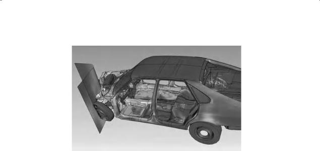
In solving partial differential equations, the primary challenge is to create an equation that approximates the equation to be studied, but is numerically stable, meaning that errors in the input and intermediate calculations do not accumulate and cause the resulting output to be meaningless. There are many ways of doing this, all with advantages and disadvantages. The FEM is a good choice for solving partial differential equations over complicated domains, like cars and oil pipelines, when the domain changes, as during a solid-state reaction with a moving boundary, when the desired precision varies over the entire domain or when the solution lacks smoothness. For instance, in a frontal crash simulation it is possible to increase the prediction accuracy in important areas like the front of the car and decrease it in its rear, thus reducing the cost of the simulation. Another example would be the simulation of the weather pattern on Earth, where it is more important to have accurate predictions over land than over the wide-open sea. Figure 3.7 shows how a car deforms in an asymmetrical crash using finite element analysis [3].

A variety of specializations under the umbrella of mechanical engineering and aeronautical engineering – such as the automotive, biomechanical and aerospace industries – use integrated FEM in the design and development of their products. Several modern FEM packages include specific components such as structural, thermal, fluid and electromagnetic environments. In a structural simulation, FEM helps tremendously in producing stiffness and strength visualizations and also in minimizing weight, materials, and costs. FEM allows a detailed visualization

Figure 3.7 Visualization of how a car deforms in an asymmetrical crash using finite element analysis (Pelosi [3])

of the sections where structures bend or twist, and indicates the distribution, stresses, and displacements. FEM software provides a wide range of simulation options for controlling the complexity of the modelling and analysis of a system. Similarly, the desired level of accuracy, and the associated computational time required, can be managed simultaneously to address most engineering applications. FEM allows entire designs to be constructed, refined and optimized before the item is manufactured.

This powerful design tool has significantly improved the standard of engineering designs and the methodology of the design process in many industrial applications. The introduction of FEM has substantially decreased the time required to take items from their conception to the production line. It is primarily through improved initial prototype designs using FEM that testing and development have been accelerated. The overall benefits of FEM include increased accuracy, enhanced design and better insight into critical design parameters, virtual prototyping, fewer hardware prototypes, a faster and less expensive design cycle, increased productivity and increased revenue.

3.7Boundary Element Method

The boundary element method (BEM) is a numerical computational method of solving linear partial differential equations which have been formulated as integral equations, that is, in boundary integral form. It can be applied to many areas of engineering and science including acoustics, fluid mechanics, fracture mechanics, electromagnetics.

The integral equation may be regarded as an exact solution of the governing partial differential equation. The BEM attempts to use the given boundary conditions to fit boundary values into the integral equation, rather than values throughout the space defined by a partial differential equation. Once this is done, the integral equation can then be used again in the postprocessing stage to calculate numerically the solution directly at any desired point in the interior of the solution domain.

The BEM is applicable to problems for which Green’s function can be calculated. As these usually involve fields in linear homogeneous media, that places considerable restrictions on the range and generality of problems to which boundary elements can usually be applied. Nonlinearities can be included in the formulation, although they will generally introduce volume integrals which then require the volume to be discretized before a solution can be attempted, removing one of the most often-cited advantages of BEM. A useful technique for treating the volume integral without discretizing the volume is the dual-reciprocity method. The technique approximates part of the integrand using radial basis functions (local interpolating functions) and converts the volume integral into a boundary integral after collocating at selected points distributed throughout the volume domain (including the boundary). In the dual-reciprocity BEM – although there is no need to discretize the volume into meshes – unknowns at chosen points inside the solution domain are involved in the linear algebraic equations approximating the problem being considered.

The Green’s function elements connecting pairs of source and field patches defined by the mesh form a matrix, which is solved numerically. Unless the Green’s function is well behaved (at least for pairs of patches near each other), the Green’s function must be integrated over either or both the source patch and the field patch. The form of method in which the integrals over the source and field patches are the same, is called Galerkin’s method. Galerkin’s method is the obvious approach for problems that are symmetrical with respect to exchanging the source and field points. In the frequency domain of electromagnetics, this is assured by electromagnetic reciprocity. The cost of computation involved in naive Galerkin implementation is typically quite severe. One must loop over elements twice and for each pair of elements we loop through Gauss points in the elements, producing a multiplicative factor proportional to the number of Gauss points squared. Also, the function evaluations required are typically quite expensive, involving trigonometric/hyperbolic function calls. Nonetheless, the principal source of the computational cost is this double-loop over elements producing a fully populated matrix.

The Green’s functions or fundamental solutions are often problematic to integrate as they are based on a solution of the system equations subject to a singularity load (e.g., the electrical field arising from a point charge). Integrating such singular fields is not easy: for simple element geometries (e.g. planar triangles), analytical integration can be used, and for more general elements it is possible to design purely numerical schemes that adapt to the singularity, but at great computational cost. Of course, when the source point and the target element (where the integration is done) are far apart, the local gradient surrounding the point need not be quantified exactly and it becomes possible to integrate easily due to the smooth decay of the fundamental solution. It is this feature that is typically employed in schemes designed to accelerate the calculations in boundary element problems.

3.7.1Comparison to Other Methods

The BEM is often more efficient than other methods, including the FEM, in terms of computational resources for problems where there is a small surface/volume ratio [8]. Conceptually, the BEM works by constructing a mesh over the modelled surface. However, for many problems BEMs are significantly less efficient than volume-discretization methods (FEM, finite difference method, finite volume method).

Boundary element formulations typically give rise to fully populated matrices, which means that the storage requirements and computational time tend to grow according to the square of

the size of the problem. By contrast, finite element matrices are typically banded, the elements are only locally connected, and the storage requirements for the system matrices typically grow quite linearly with the size of the problem.

References

[1]Cooley, J.W. and Tukey, J.W. (1965) An algorithm for the machine calculation of complex Fourier series. Math. Comput., 19(90), 297–301.

[2]Jain, A.K. (1989) Fundamentals of Digital Image Processing, Prentice Hall, New Jersey.

[3]Pelosi, G. (2007) The finite-element method, Part I: R.L. Courant: Historical Corner. IEEE Antennas. Propag. Mag., 49, 180–182. doi: 10.1109/MAP.2007.376627

[4]Wikipedia (2011) http://en.wikipedia.org/wiki/Beamforming, Accessed 2011.

[5]Stein, E. and Zienkiewicz, O.C. (2009) A pioneer in the field of the finite element method in engineering science.

Steel Construction, 2(4), 264–272.

[6]Weaver, W. Jr. and Gere, J.M. (1966) Matrix Analysis of Framed Structures, 3rd edn, Springer-Verlag, New York.

[7]Strang, G. and Fix, G. (1973) An Analysis of the Finite Element Method, Prentice Hall, New Jersey.

[8]Gibson, W.C. (2008) The Method of Moments in Electromagnetics, Chapman & Hall/CRC, Florida, USA.