акустика / gan_ws_acoustical_imaging_techniques_and_applications_for_en

The aforementioned assumptions (a) and (b) correspond to near-field or Fresnel approximation, meaning that the acoustic transmitters and receivers are fairly chose to each other for reflection mode imaging or on opposite sides of the object for transmission mode imaging. In the third assumption (c), if z were very large compared to the acoustic aperture, then only the first term z would be retained to give the far-field or Fraunhofer approximation. The assumption in approximation (11.7) corresponds to the near-field or Fresnel region between approximately D and D2/ λ.

Substituting these approximations in equation (11.6) gives

has been made.

The resulting integral in equation (11.8) is a Fourier transform of the term in brackets. The new variables fx and fy can be interpreted as spatial frequencies across the array. This

is for broadband case, since A, fx and fy depend on frequency ω. We first discuss single frequency system.

Taking the inverse Fourier transform of (11.8), we have

Here A0 is the same as A mentioned previously except for x0 and y0 replacing x and y, respectively. Equation (11.10) is again a spatial Fourier transform of the term in brackets. That is, with the exception of the A0 term and the exponential inside the brackets, the image signal at any point can be calculated by a Fourier transform of the array signals. The term A0 is made up of

(a)a constant ω/ 2π c,

(b)a 1/z term that accounts for spherical spreading loss,

(c)a phase term exp [ jωz/c] that represents the mean phase shift of the signal as it propagates near the range z and

(d)a quadratic phase term exp[ jω(x02 + y20 )/2cz] that compensates for the assumption that the target plane was to be flat when it is actually spherical.

Terms (a) and (b) are attenuation factors. Terms (c) and (d) are phase factors that will disappear on taking the intensity of the image. Hence, A0 can be ignored.

The quadratic phase factor inside the bracket is the so-called Fresnel focus factor, which must be applied to the observed data just prior to Fourier transforming. The result is the acoustic image of the target.

In simpler form,

where k = ωc = 2λπ and time has been neglected. This is the basis on which many singlefrequency sonar beamformers and image systems are designed.

The quadratic Fresnel phase factor is the focusing mechanism. At a given range z, the range

The aforementioned analysis can also be given by the technique of backward propagation. Backward propagation does not use the Fresnel approximation and hence, is applicable even in the very near field of the array. Using backward propagation approach, equation (11.10) can be rewritten as

−∞

where

h (x, y, z; x0, y0 ) = ω exp ( jωr/c) cos(n, r). j2π cr

Using the approximation given by equations (11.7a) and (11.7b), h becomes

which is a spatial convolution and equation (11.14) becomes

By taking the Fourier transform of both sides, the convolution becomes

Thus, backward propagation consists of the following steps:

(a)Take the Fourier transform of the array data.

(b)Multiply by H−1 ( fx, fy ) at a fixed z.

(c)Take the inverse Fourier transform of the result to produce the image.

11.4Characteristics of Underwater Acoustical Imaging Systems

First of all, underwater acoustical imaging has a different way of image formation from conventional side-scan sonars and sector-scan sonars. For instance, sector-scan sonars display reflected acoustic intensity on a polar plot of bearing versus range. An object on the bottom appears on the display as a bright spot, backed by a two-dimensional shadow. A side-scan sonar produces a rectangular display that is very similar. For certain geometries these systems produce very good images of objects on the ocean floor. Underwater acoustical imaging systems generally produce images in a vertical plane similar to that used in optical imaging system, that is, reflected energy versus vertical and lateral direction at some range.

The characteristics of underwater acoustical imaging are different from that of other branches of acoustical imaging such as medical ultrasound imaging and ultrasound nondestructive testing as can be shown by the following parameters:

Hence, there are major differences in range spread of interest, geometries that are practical and techniques that can be used. Because of these differences, the techniques and results from one field are not directly transferable to another. For instance, the units of resolution used here is angular resolution subtended by a minimally resolvable dimension at some range. This is due to the great spread of ranges that are of interest in these applications. It is given by λ/D, where λ is the sound wavelength and D is the receiving aperture diameter. The maximum range in seawater is limited at the upper frequencies by the attenuation coefficient of seawater and at all frequencies by spherical spreading loss. The depth of field of the imaging system depends on the focusing capability of the imaging system, the properties of the acoustic receiver and the

duration of the acoustic signals. The units of resolutions used in medical ultrasound imaging and ultrasound nondestructive testing are minimum resolvable distances.

Underwater acoustical imaging systems normally work within the Fresnel region or the far-field region. In this region, spherical waves radiating from a point source can be treated as plane waves and no focusing is necessary and it begins at a range of D2/λ. The Fresnel region extends down to a range of D or 2D from the aperture. In this near-field region, the sound wave phase has to be taken into account. Focusing is needed here as what is done in geometrical optics. The underwater acoustic imaging systems have the ability to focus at different ranges and to tolerate out-of-focus images.

Most underwater acoustical imaging systems and sonars use narrow bandwidth acoustic signals. They are used due to the following reasons: (1) single frequencies are easier to generate with existing acoustic transducer design and (2) they are necessary to accomplish the signal processing. This is because these systems approximate time delay by the phase shift of a sine wave signal. Use is made of the following properties: (1) two or more sine waves add up to form a new sine wave and (2) sine waves repeat. These narrow bandwidth acoustic signals give rise to the undesirable speckle, a problem also encountered by optical holography with lasers. Speckle is due to the mutual interference of the signal from one part of the target with that from another part. This gives rise to bright and dark areas in the image that are on the same order of size as the details of the object being imaged but are not related to any detail on the object. Hence, speckles tend to be very confusing and distracting.

With broadband signals, the speckle patterns due to the different frequency components tend to cancel each other, leaving more uniform and representative image information. For systems like focused beamformers and delay-and-sum beamformers, the signal processing techniques are independent of frequency over a wide bandwidth.

Other characteristics of underwater acoustical system are: properties of the platform, environmental requirements on the hardware and typical target properties. An acoustic imaging system must be insensitive to platform motion and it must produce images at a frame rate sufficiently fast to provide useful, timely results to the vehicle operators. Most underwater platforms impose restrictions on size, weight and power available for the system.

Environmental requirements on the underwater imaging system might also be severe, especially if it is to be used at sea. Except for the ambient pressure of water, the most severe stresses are not applied when the system is actually in use. Vibration stresses are applied during transit to the operating site aboard a surface vessel. Shock stresses are worst during launching of the entire platform/sensor system through the air–sea interface due to wave slap and slip roll. Also, in an ocean environment, corrosion must also be taken into account. In general, the techniques that compensate for these environmental hazards affect system size, weight and cost, but do not significantly affect performance.

Target properties play a part in underwater acoustical imaging. There are many objects on the bottom of the ocean that could appear in an acoustic image, including many that are not of interest but could appear brighter than the ones of interest. For instance, the bottom itself is usually in the image unless steps are taken to filter it out. Another consideration in target properties is that the objects are partially transparent. Sound nearby always penetrates objects, reflecting from inner and back surfaces to produce multiple echoes and interfering internal reflections. This effect, called ‘ringing’, provides additional information about the target while complicating the interpretation of the acoustic image.

(a)

(b)

(c)

Figure 11.5 Sonar imaging. (a) Geometry showing acoustic return from bottom and object, but none from shadow behind object. (b) A-scan or oscilloscope trace of received sonar signal versus time. (c) Resulting sonar shadow image from many narrow sonar beams as shown in PPI display (Lee and Wade [8] © IEEE)

sonar (SLS) and (3) synthetic aperture side-looking sonar. SLS and synthetic aperture sidelooking sonar form images by transmitting a beam of sound at a grazing angle to the bottom (refer to Figure 11.5) when no object is present. The bottom backscatters the energy as a more- or-less uniform background. When an object is present and rests above the bottom, it intercepts and reflects some of the energy earlier than the bottom. Hence, more energy is reflected to form a bright spot at the range of the object. Meanwhile, no energy is reflected by the bottom within the shadow of the object. As the beam is scanned across the field of view, the beam interacts with different parts of the object. Hence, the shadow of the object appears on the display screen just beyond the bright spot. The bright spot indicates the presence of something, the shadow indicates the shape of it. The sector-scan sonar has a plan-position indicator (PPI) type of display, which is essentially a portion of a polar coordinate plot. The display may be generated by a single swept beam or multiple performed beams. The SLS produces one line at a time in a rectangular display format. In this case, only one beam is transmitted perpendicularly out

Figure 11.6 Side-look sonar image of a sunken vessel (Lee and Wade [8] © IEEE)

to the side at any one time. The spatial converge is obtained by moving the sonar physically through the water, perpendicular to the direction of sound transmission. Thus, it too sweeps a beam across the object to form a bright spot/shadow display of the object. An example of an SLS image of a sunken vessel is shown in Figure 11.6.

The synthetic aperture side-looking sonar uses a wider beam and by means of accurate navigation, coherently combines the returns from several transmit cycles to form each display beam. Thus, the effect is similar to that of the SLS.

11.5.2Orthoscopic Acoustical Imaging

This type of imaging modality forms the images in a lateral versus vertical format, similar to that of the optical imaging. There are four methods of imaging here. These four methods all follow the following procedures:

Spatial processing to derive an image from the acoustic field.

Transduction to change from acoustic energy to electrical energy.

Detection to convert high-frequency signals to an observable, near-DC image signal and some form of display.

These four methods differ only in the order in which they perform these steps. Their imaging procedures are as follows:

(a)Focused acoustical imaging use an acoustic lens or reflector to focus high-frequency sound image onto an acoustic retina, much like a TV camera focuses light images into an optical retina. That is, they perform spatial processing first, followed by transduction and detection.

(b)Beamformed acoustical imaging performs transduction then the spatial processing electronically. This eliminates the need for an acoustic lens.

(c)In the holographic approach, the transduction and detection are performed first to produce an acoustical hologram. Then spatial processing or reconstructing the hologram is

performed, allowing the processing to be performed at baseband rather than at the acoustic frequency.

(d)In Bragg imaging laser light interacts directly with the water volume to produce observable optical images.

The techniques available for each of the functions and certain physical constraints determine which particular type of system is best in a given application.

For the aforementioned imaging modalities, there are necessary choices of hardware techniques to choose from for the implementation of spatial processors detection, displays, source–receiver configuration and predetection and postdetection signal processing. These can be referred to the series of proceedings on acoustical imaging.

An underwater acoustical imaging system uses filled, two-dimensional planar array of hydrophones for the detection of underwater signals. A broad-beamed acoustic source is used.

Synthetic aperture technique is also used. It means the simulation of a filled array by the clever use of some smaller array. Examples include a line array scanned perpendicular to its length, a point transducer scanned in a raster and many other schemes. The idea is to replace the large array of receiving transducers with a smaller number of sensors in some scanning arrangement. The price to be paid for the savings in transducers may include increased scan time, which can lead to motion blurring and slower frame rate or lower signal-to-noise ratio.

11.6 A Few Representative Underwater Acoustical Imaging System

11.6.1Focused Acoustical Imaging System

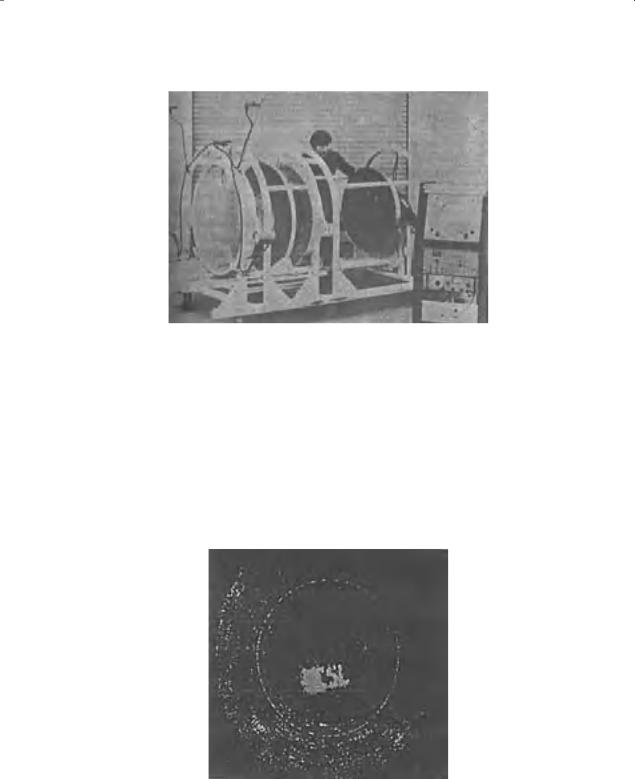
This system design is analogous to geometrical optics system and an acoustic lens is used for focusing the sound beam. The advantage of the system is simplicity, sheer size and inherently broadband nature. The acoustic array and signal processing electronics are fairly simple since one only needs to detect the amplitude (or intensity) of the incident acoustic energy. Acoustic lens requires some distance between itself and the focal plane, and this gives rise to huge size and bulkiness. This is expected true for thin lens but less so for spherical lens. An example of the focused underwater acoustical imaging system is shown in Figure 11.7. The system in Figure 11.7 is developed by the Naval Coastal System Centre in Panama City, FL, USA.

This system consists of a 1-metre diameter, temperature-corrected six-element acoustic lens on a movable focusing framework, a rotating line array of hydrophones and their corresponding signal amplification/detection circuitry and a display screen. The acoustic lens focuses the acoustic energy onto the receiving plane, while the rotating line receiver scans out the image to the display.

Four separate acoustic projectors transmit acoustic energy into the water to obtain diffuse illumination. The system has a range of 10–150 m and a resolution of 0.12 degree, at a frequency of operation of 860 kHz. Figure 11.8 is an image of the letters NCSL on the display tube. Frame rate is one per second. The performance of the system is analogous to that of an underwater TV camera. Other research centres on focused underwater acoustical imaging systems in the United States are: (1) Westinghouse Research Labs and research centres, using spherical lenses and Luneberg lenses such as (2) Autonetics division of Rockwell International,

(3) Naval Ocean Systems Centre and (4) Applied Physics Lab, University of Washington.

Figure 11.7 A focused underwater acoustic imaging system using a six-element, temperature-corrected lens and a rotating line array of receivers. The four projections at the front are acoustic sources (Lee and Wade [8] © IEEE)

11.6.2Electronic Beam-Focused Underwater Acoustical Imaging System

Beamforming systems are a bit more complicated than focused systems. Beanforming means the combination of the acoustic signals from several transducers into beams, followed by detection of the energy in each beam. These systems vary from a single pencil beam scanned in a raster fashion across the field of view to multiple preformed beams that observe the entire field of view at one time. They encompass actual physical beams of sound transmitted into the

Figure 11.8 Acoustic image of the 18-inch tall letters ‘NCSL’ made of pipes taken at 30 m with a focused system (Lee and Wade [8] © IEEE)

D = Nd

Figure 11.9 Geometry and nomenclature of a horizontal line array of hydrophones with acoustic wavefronts impinging from the upper right (Lee and Wade [8] © IEEE)

water as well as the separation of received signals into electronic paths that represent virtual beams. By combining acoustic signals from many acoustic transducer elements, acoustic beams of various shapes (usually pencil or fan beams) can be generated in the water and scanned over the field of view. As the beams scan across the field of view, the received intensity is measured and displayed in a corresponding geometry.

There are three basic classes of beamformers: (1) delay and sum, (2) phased array and (3) correlation.

11.6.2.1Delay and Sum Beamformer

The delay and sum beamformer is best typified by time delays and summing amplifiers. The delay for each image element is chosen to compensate for the acoustic path delay.

To understand the geometry of a regularly spaced line array, one must consider Figure 11.9. For θ = 0, array steered broadside, all of the acoustic wavefront arrive simultaneously. So no delays are applied. When θ = 0, as shown in Figure 11.9, the wavefront arrives at transduce N − 1 first, then at N − 2, and so forth down the array. In order for each receiver channel to detect this signal at the proper time, succeedingly longer time delays must be introduced at each subsequent channel. The net result is that the output of the lth beam Sl , is given by

where gk is the signal at the kth hydrophone at time t. The amount of increase in time delay between two adjacent channels is tl = d sin θl /c.

To form one beam in one direction requires N time delay units. To form P such beams simultaneously looking in different directions requires P × N time delays, or alternatively, N delays having P taps each. It has the desirable property of being inherently a broadband system. The primary problem with this type of system is the unavailability of high-speed short-term