

FinMarketsTrading
.pdfInventory Models |
29 |
Price
λb (p)
λa (p)
Ask
Bid
λopt |
Arrrival rate |
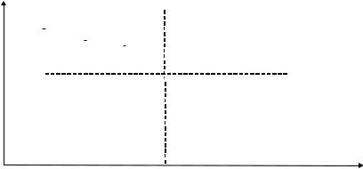
FIGURE 3.1 Dealers’ profits in the Garman’s model for the case (3.10).
A m i h u d - M e n d e l s o n M o d e l
One significant simplification of the Garman’s model is that the dealer establishes pricing in the beginning of trading and does not adjust it to everchanging market conditions. This problem was addressed by Amihud & Mendelson (1980) by reformulating the Garman’s model so that bid and ask prices depend on the dealer’s stock inventory. More specifically, the dealer has an acceptable range and a preferred size of the inventory. The dealer maximizes trading profits by manipulating the bid/ask prices when inventory deviates from preferred. Amihud & Mendelson obtain their main results for linear demand and supply functions. Within their model, optimal bid and ask prices decrease (increase) monotonically when inventory is growing (falling) beyond the preferred size. The bid/ask spread increases as inventory increasingly deviates from the preferred size (see Figure 3.2). The practical conclusion from the Amihud-Mendelson model is that dealers should manipulate the bid/ask spread and mid-price for maintaining preferred inventory.
M O D E L S W I T H R I S K A V E R S I O N
W h a t I s R i s k A v e r s i o n ?
The concept of risk aversion is widely used in psychology, economics, and finance. It denotes an individual’s reluctance to choose a bargain
30 |
|
|
|
|
|
|
|
|
|
|
|
|
|
|
MARKET MICROSTRUCTURE |
|||||
Price |
|
|
|
|
|
|
|
|||||||||||||
Pa |
|
|
|
|
|
|
|
|
|
|
|
|
|
|
|
|
|
|
Pa |
|
Pb |
|
|
|
|
|
|
|
|
|
|
|
|
|
|
|
|
|
|
|
|
|
|
|
|
|
|
|
|
|
|
|
|
|
|
|
|
|
|
|
||
|
|
|
|
|
|
|
|
|
|
|
|
|
|
|
|
|
|
|
||
|
|
|
|
|
|
|
|
|
|
|
|
|
|
|
|
|
|
|
|
Pb |
|
|
|
|
|
|
|
|
|
|
|
|
|
|
|
|
|
|
|
|
|
|
|
|
|
|
|
|
|
|
|
|
|
|
|
|
|
|
|
|
|
|
|
|
|
|
|
|
|
|
|
|
|
|
|
|
|
|
|
|
|
|
|
|
|
|
|
|
|
|
|
Preferred position |
|
|
|
|
|
|
Inventory |
|||||
|
|
|
|
|
|
|
|
|
|
|
|
|
|
|
|
|
|
|
|
level |
FIGURE 3.2 The dependence of bid and ask prices in the Amihud-Mendelson model.
with uncertain payoff over a bargain with certain but possibly lower payoff. Risk aversion is routinely observed in everyday life: Just recall that we put much of our savings in a bank, money market, or CDs rather than invest them in the ever volatile yet potentially rewarding equity market.
The concept of risk aversion was empirically tested and theoretically advanced in studies of behavioral finance, the field that focuses on psychological and cognitive factors that affect people’s financial decisions (see Kahneman & Tversky, 2000, for a review). In widely popularized experiments with volunteers, Kahneman and Tversky suggested making choices in two different situations. First, participants assumed to have $1,000 and were given a choice between (1) gambling with 50 percent chances to gain $1,000 and 50 percent to gain nothing, or (2) sure gain of $500. In the second situation, participants assumed to have $2,000 and were given a choice between (1) 50 percent chance to lose $1,000 and 50 percent to lose nothing and (2) sure loss of $500. In both situations, option 2 guaranteed a gain of $1,500. Hence, risk-neutral participants would split equally between these two situations. And yet, the majority of participants chose option 2 in the first situation and option 1 in the second situation. Such an outcome implies that the majority of participants were riskaverse.
In classical economics, utility functions U(W) of wealth W are used for quantifying risk aversion. The notion of utility function is rooted in the efficient market hypothesis, according to which investors are rational and act exclusively for maximizing their wealth (see Chapter 7). Findings in behavioral finance indicate that the utility function generally is not linear
Inventory Models |
31 |
upon wealth. One of the widely used utility functions is the constant absolute risk aversion (CARA):
UðWÞ ¼ expð aWÞ |
ð3:11Þ |
The parameter a is called the coefficient of absolute risk aversion. The important property of CARA is that its curvature is constant:
zCARAðWÞ ¼ U00ðWÞ=U0ðWÞ ¼ a |
ð3:12Þ |
While it is relatively easy to use CARA in theoretical analysis, absolute aversion may not always be an accurate assumption. Indeed, the loss of $1,000 may be perceived quite differently by a millionaire and a college student. Then the constant relative aversion function (CRRA) can be used:
UðWÞ ¼ when |
a ¼6 1 |
ð3:13Þ |
¼ lnW when |
a ¼ 1 |
|
In this case, the coefficient of relative risk aversion is constant: |
|
|
zCARAðWÞ ¼ WU00ðWÞ=U0ðWÞ ¼ a |
ð3:14Þ |
|
T h e S t o l l ’ s M o d e l
The Amihud–Mendelson model implies dealer’s risk aversion in that he focuses on reducing deviations from preferred inventory. Stoll (1978) was the first to explicitly introduce the concept of risk aversion in the inventory models. In the Stoll’s model, the dealer modifies his original portfolio (which is efficient in terms of CAPM4) to satisfy demand from liquidity traders in asset i and compensates his risk by introducing the bid/ask spread. Stoll considered a two-period model in which the dealer makes a transaction at time t ¼ 1 and liquidates this position at t ¼ 2. The price may change between (but not within) the trading periods. The main idea behind Stoll’s approach is that the dealer sets such prices that his expected CARA utility function of the entire trader’s portfolio does not change due to trading of the asset i
E½UðWÞ& ¼ E½UðWT Þ& |
ð3:15Þ |
In (3.15), W and WT are the terminal wealth of the initial portfolio W0 and the terminal wealth of the portfolio after transaction, respectively:
W ¼ W0ð1 þ rÞ |
ð3:16Þ |
WT ¼ W0ð1 þ rÞ þ ð1 þ riÞQi ð1 þ rf ÞðQi CiÞ |
ð3:17Þ |

32 |
MARKET MICROSTRUCTURE |
Here, r, ri, and rf are rates of return for the entire portfolio, for the risky asset i, and for the risk-free asset, respectively5; Qi is the true value of the transaction in asset i; Ci is the present value of the asset i. Hence, Stoll assumes that the dealer knows the true value of the asset i. Note that Qi > 0 when the dealer buys and Qi < 0 when the dealer sells.
For the analytical solution, Stoll sets rf ¼ 0 and expands both sides of
(3.15) into the Taylor series around the mean wealth W and drops the terms of order higher than two:
E U |
W |
|
E U |
|
|
U0 W |
|
|
0:5U00 |
|
|
|
|
|
|
2 |
|
|
|
Þ& |
W |
Þ& þ |
W |
Þ þ |
ð |
W |
|
W |
ð |
3:18 |
Þ |
||||||||
½ ð |
|
½ ð |
|
ð |
|
|
|
Þ |
|
|
|||||||||
The asset return is assumed to have the normal distribution |
|
|
|
||||||||||||||||
|
|
|
|
|
W ¼ NðW0; spÞ |
|
|
|
|
|
|
|
ð3:19Þ |
||||||
Ultimately, this yields the relation |
|
|
|
|
|
|
|
|
|
|
|
|
|
||||||
|
ciðQiÞ ¼ Ci=Qi ¼ zsipQp=W0 þ 0:5zsi2Qi=W0 |
ð3:20Þ |
|||||||||||||||||
where z is the coefficient of relative risk aversion (3.14), sip is the covariance between the asset i and the initial portfolio, Qp is the true value of the original portfolio, and si2 is variance of the asset i. If the true price of the asset i is Pi , then the prices of the immediacy to sell Qbi to (to buy Qai from) the dealer Pbi (Pai ) satisfy the relations
ðPi PibÞ=Pi ¼ ciðQibÞ |
ð3:21Þ |
ðPi PiaÞ=Pi ¼ ciðQiaÞ |
ð3:22Þ |
Then the bid/ask spread is defined from the round-trip transaction for j Qai j ¼ j Qbi j ¼ jQj
ðPia PibÞ=Pi ¼ ciðQibÞ ciðQiaÞ ¼ zsi2jQj=W0 |
ð3:23Þ |
This spread depends linearly on the dealer’s risk aversion, trading size, and asset volatility, but is independent of the initial inventory of the asset i. However, bid and ask prices are affected with the initial asset inventory: the higher the inventory is, the lower the bid and ask prices are.
An obvious shortcoming of the Stoll’s model is that it assumes complete liquidation of the asset position at t ¼ 2. Stoll’s original work was expanded by Ho and Stoll (1981) into a multi-period framework. In this work, the true trading asset value is fixed while both order flow and portfolio returns are stochastic. Namely, order flow follows the Poisson process and return is a Brownian motion with drift. The dealer’s goal is to maximize utility of his wealth at time T. This problem can be solved using the methods of dynamic programming.6 The intertemporal model shows that the optimal bid/ask
Inventory Models |
33 |
spread depends on the dealer’s time horizon. Namely, the closer to the end of trading, the smaller is the bid/ask spread. Indeed, as duration of exposure to risk of carrying inventory decreases, so does the spread being the compensation for taking risk. In general, the spread has two components. The first one is determined by specifics of supply and demand curves (assumed to be linear by Ho & Stoll, and the second one is an adjustment due to the risk the dealer accepts by keeping inventory. This adjustment depends on the same factors as the spread in the Stoll’s one-period model (3.23): risk aversion, price variance, and the size of transaction. Also, similar to the two-period model, the spread is independent of the asset’s inventory size.
Ho & Stoll (1983) offered another generalization of the Stoll’s model that describes the case with competing dealers. Namely, dealers in this work can trade among themselves and with liquidity traders. It is assumed that dealers can have varying endowments but they have the same risk aversion. Liquidity traders trade with the dealer(s) that offer the best price. When several dealers offer the best price, the matching dealer is chosen randomly. The bid/ask spread in this model, too, depends on the product zsi2jQj [see (3.23)] and it decreases with the growing number of dealers.
An interesting point indicated by Ho & Stoll (1983) is that trading fees are reflected by the second best prices rather than by the prices on top of the order book. Indeed, say the best bid price is B1 and the second best price is B2 < B1. Then the first dealer can decrease his price to B2 þ e < B1 (where e is an infinitesimal increment) and still remain on top of the book. The importance of the second best price has some parallel with the Vickrey’s auction, in which bidders submit sealed bids and a bidder with the highest bid wins; yet, the winner pays the second high bid rather than his own price.
O’Hara (1995) and de Jong & Rindi (2009) provide detailed reviews of inventory market models.
SUMMARY
&Inventory models address the dealer’s problem of maintaining inventory on both sides of the market. Since order flows are not synchronized, dealers face the possibility of running out of cash (bankruptcy) or out of inventory (failure).
&Risk-neutral models (Garman 1976; Amihud & Mendelson 1980) are based on the Walrasian framework according to which lower (higher) price drives (depresses) demand. These models demonstrate that rational dealers attempting to maximize their

34 |
MARKET MICROSTRUCTURE |
profits must establish a certain bid/ask spread and manipulate its size for maintaining preferred inventory.
&Risk aversion is a concept that refers to an individual’s reluctance to choose a bargain with uncertain payoff over a bargain with certain but possibly a lower payoff.
&In mathematical terms, risk aversion is usually described with some utility function that is non-linear upon wealth. Inventory models with risk aversion are based on optimizing this utility function.
&The basic two-period inventory model offered by Stoll (1978) considers a single dealer who optimizes the CARA utility function (3.11) and assumes that the return of a risky asset has the normal distribution. This model yields the bid/ask spread that depends linearly on the dealer’s risk aversion, trading size, and the asset volatility.
&Extensions of the Stoll’s model for multi-period framework and for competing dealers (Ho & Stoll 1981, 1983) retain linear dependence of the bid/ask spread on risk aversion and volatility. In the multi-period model, the optimal spread narrows since the risk for maintaining inventory diminishes as trading comes to the end. The spread also decreases with the growing number of competing dealers as the risk is spread among them.

Financial Markets and Trading: An Introduction to
Market Microstructure and Trading Strategies by Anatoly B. Schmidt Copyright © 2011 Anatoly B. Schmidt
CHAPTER 4
Market Microstructure:
Information-Based Models
The idea behind the information-based models of market microstructure is that price is a source of information that investors can use for their trading decisions (see O’Hara 1995 and de Jong & Rindi 2009, for a detailed review). For example, if security price falls, investors may suggest that price will further deteriorate and refrain from buying this security. Note that such a behavior contradicts the Walrasian paradigm of market equilibrium,
according to which demand grows (falls) when price decreases (increases). The information-based models are rooted in the rational expectations
theory. Namely, informed traders and market makers make conjectures on rational behavior of their counterparts, and they do behave rationally in the sense that all their actions are focused on maximizing their wealth (or some utility function in the case of risk-averse agents). Market in these models reaches an equilibrium state that satisfies participants’ expectations. Obviously, informed investors trade only on one side of the market at any given time. The problem that market makers face while trading with informed investors is called adverse selection.
In this chapter, I consider two information-based models that were introduced for describing two different markets. The first is the Kyle’s (1985) model, which was developed for batch auction markets. Another model is offered by Glosten & Milgrom (1985) to address the adverse selection problem in sequential trading.
K Y L E ’ S M O D E L
O n e - P e r i o d M o d e l
Kyle (1985) considers a one-period model with a single risk-neutral informed trader (insider) and several liquidity traders who trade a single risky security
35

36 |
MARKET MICROSTRUCTURE |
with a risk-neutral market maker (dealer). The batched auction setup implies that the market clears at a single price. Hence, the bid/ask spread is irrelevant. The informed trader (insider) knows that the security value in the end of the period has the normal distribution
v ¼ Nðp0; s02Þ |
ð4:1Þ |
The insider trades strategically, that is, submits an order of size x(v) to optimize her profits in the end of the period. Liquidity traders submit their orders randomly and their total demand y is described with the normal distribution
y ¼ Nð0; sy2Þ |
ð4:2Þ |
Both random variables v and y are independently distributed. The dealer observes the aggregate demand, z ¼ x þ y, but is not aware what part of it comes from the informed trader. The dealer sets the clearing price p(z) that is expected to optimize his profits. Naturally, p(z) increases with growing aggregate demand. The insider’s profit equals
pI ¼ xðv pÞ |
ð4:3Þ |
Kyle obtains the equilibrium price (i.e., the price that yields the optimal profits for both dealer and insider) analytically for the case when the clearing price depends linearly on demand:
pðzÞ ¼ lz þ m |
ð4:4Þ |
In (4.4), l characterizes inverse liquidity. Indeed, lower l (higher liquidity) leads to lower impact of demand on price. Sometimes, inverse liquidity is called illiquidity (see Eq. (1)). It follows from (4.3) and (4.4) that
E½pI& ¼ xðv lx mÞ |
ð4:5Þ |
As a result, the optimal insider’s demand equals
x ¼ ðv mÞ=2l |
ð4:6Þ |
Another form of (4.6) is
x ¼ a þ bv; a ¼ m=2l; b ¼ 1=2l |
ð4:7Þ |
Then, all variables of interest can be expressed in terms of the model parameters (p0, s0, and sy). Indeed, since v and z have normal distributions, it can be shown that E[vjz] has the following form1
E v z |
p |
|
þ |
bðz a bp0Þs02 |
ð |
4:8 |
Þ |
|
sy2 þ b2s02 |
||||||
½ j & ¼ |
|
0 |
|
Market Microstructure: Information-Based Models |
37 |
In equilibrium, the right-hand sides of (4.4) and (4.8) must be equal for all z. Then
a ¼ p0sy=s0; b ¼ sy=s0; |
ð4:9Þ |
m ¼ p0; |
ð4:10Þ |
l ¼ s0=2sy |
ð4:11Þ |
The equality (4.10) m ¼ p0 ¼ E[vjz ¼ 0] implies that the dealer sets price at its mean (true) value in case of zero demand. Note also that the inverse liquidity in equilibrium (4.11) is determined with variances of price and demand.
An interesting property of the Kyle’s model is that price variance conditional on the aggregate demand equals
VarðvjzÞ ¼ s02=2; |
ð4:12Þ |
which is only one half of the unconditional price variance. The result (4.12) implies that the order flow provided by liquidity traders distorts the information available to informed traders. Indeed, even if an insider knows that the traded security is overpriced and hence is not interested in buying it, a large idiosyncratic buy order from a liquidity trader will motivate the dealer to increase the price.
Now, consider profits and losses of all market participants. It follows from (4.5) that the expected insider’s profit equals
E½pI& ¼ 0:5sys0 |
ð4:13Þ |
Note that only the expected insider’s profit is positive. In fact, insiders may experience a loss according to (4.3), when the idiosyncratic rise of demand from liquidity traders leads to the condition v – lz – m < 0. The trading cost of liquidity traders turns out to be equal to the insider’s profit (de Jong & Rindi 2009)
E½pL& ¼ E½yðp vÞ& ¼ lsy2 ¼ 0:5sys0 |
ð4:14Þ |
Hence, the expected insider profits are funded with losses incurred by liquidity traders. The total dealer’s profits in the Kyle’s model are zero. The (sufficiently) good news is that the dealer has no losses. There is a general rationale for expecting the dealer’s zero profits (unless he is monopolistic). The so-called Bertrand competition model demonstrates that competing businesses inevitably lower the price on their product until the price reaches the product marginal cost. Why then does anyone bother to run batch auctions? Firstly, auction owners receive transaction fees. And secondly, a constantly informed trader is just an abstraction.

38 |
MARKET MICROSTRUCTURE |
M u l t i - P e r i o d a n d M u l t i - I n s i d e r M o d e l s
Kyle (1985) considers also a model with K auctions that are held at times tk ¼ kDt ¼ k/K; k ¼ 1, 2, . . . , K. Note that the discrete model approaches a continuous auction when Dt ¼ 1/K decreases. It is assumed that the order flow from liquidity traders follows the Brownian motion: Dyk ¼ N(0, sy2Dt). The insider’s demand is
Dxk ¼ bkðv pkÞDt |
ð4:15Þ |
The dealer sets a price that depends linearly on total demand:
pk ¼ pk 1 þ lkðDxk þ DykÞ |
ð4:16Þ |
In the end of the auction k, the dealer’s expected profits have the form
Eðpkjp1; . . . ; pk 1; vÞ ¼ ak 1ðv pk 1Þ2 þ dk 1 |
ð4:17Þ |
In equilibrium, the coefficients in (4.15)–(4.17) satisfy the relations
|
lk ¼ bksk2=sy2 |
ð4:18Þ |
||||
b |
Dt |
¼ |
1 2aklk |
ð |
4:19 |
Þ |
k |
|
2lkð1 aklkÞ |
|
|||
ak 1 ¼ 1=½4lkð1 aklkÞ& |
ð4:20Þ |
|||||
dk 1 ¼ dk þ aklk2sy2Dt |
ð4:21Þ |
|||||
In contrast to the single-period model, the variance is now time-dependent:
sk2 ¼ ð1 bklkDtÞsk 12 |
ð4:22Þ |
Since the system of equations (4.18)–(4.22) is non-linear, an iterative procedure is needed for solving it.
In the multiple-period model, the insider splits her orders into small pieces with sizes varying with time. Such a strategy has become a standard practice in executing large orders (see Chapter 13). In the real world, this leads to positive autocorrelations in order flows, which implies some predictability of an insider’s actions. However, this is not the case in the Kyle’s model, which allows the insider to hide her orders behind uncorrelated orders submitted by liquidity traders. Ultimately, however, the price reflects the entire insider’s information and her profits are limited.