

FinMarketsTrading
.pdf
|
|
|
|
Price |
140 |
120 |
100 |
80 |
60 |
|
|
|
|
6/2/2010 |
5/2/2010 |
4/2/2010 3/2/2010
2/20102/ |
1/2/2010 12/2/2009
11/2/2009 |
10/2/2009 |
9/2/2009 |
8/2/2009 |
|
|
|
|
7/2/2009 |
|
|
|
|
6/2/2009 |
|
|
|
|
5/2/2009 |
|
|
|
|
4/2/2009 |
|
|
|
|
3/2/2009 |
|
|
|
|
2/2/2009 |
|
|
|
|
1/2/2009 |
3 |
2 |
1 |
0 |
–1 |
|
|
|
|
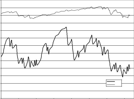
MACD |
40 |
20 |
0 |
Price
Signal line
MACD line
Histogram
|
|
|
Example of MACD for SPY. |
–2 |
–3 |
–4 |
FIGURE 10.3 |
112

Technical Trading Strategies |
113 |
Typical RSI values for the overbought/oversold markets are 70/30. An example of RSI for SPY is given in Figure 10.4. For some volatile assets, RSI reaches the overbought/oversold conditions quite frequently. Then, the RSI spread may be widened to 80/20 (Kaufman 2005).
C O M P L E X G E O M E T R I C P A T T E R N S
Trends and oscillators have relatively simple visual forms and straightforward definition. However, some other popular TA patterns, while being easily recognizable with a human eye, represent a challenge for quantitative description. These include head-and-shoulder (HaS), inverse HaS, broadening tops and bottoms, triangle tops and bottoms, double tops and bottoms, and others (Edwards & Magee 2001; Kaufman 2005). The main challenge in finding complex geometric patterns in a time series is filtering out noise that may produce false leads. The smoothing technique with kernel regression was successfully used for analysis of TA strategies by Lo et al. (2000) in equities and by Omrane & Oppens (2004) in FX.
Here, we describe HaS as an example. Visually, HaS is determined with five price extremes: three maxima that refer to two shoulders surrounding the head, and two valleys between the shoulders and the head (see Figure 10.5).
HaS has a neckline—the support line connecting the shoulder minima. The trading idea based on HaS is a selling signal when price breaks through the neckline from above. Inverse HaS is a mirror image of HaS in respect to the time axis. This pattern generates a buy signal when price breaks through the neckline from below.
Lo et al. (2000) have a relatively simple definition of HaS. Namely, HaS is determined with five consecutive extremes: E1, E2, E3, E4, and E5, such that
E1 is a maximum;
E3 > E1; E3 > E5 |
ð10:22Þ |
E1 and E5 are within 1.5 percent of their average
E2 and E4 are within 1.5 percent of their average
However, Omrane & Van Oppens (2004) define HaS with nine rules including conditions for the relative heights of the head and shoulders and timings between them. Many TA experts emphasize that the trading models should not be over-fitted (e.g., Kaufman 2005; Kerstner 2003; Lo et al. 2000). The problem with overly complicated models is that they are sensitive
114 |
130 |
|
|
|
|
|
|
|
120 |
|
|
|
|
|
|
|
|
|
|
|
|
|
|
|
|
|
|
110 |
|
|
|
|
|
|
|
|
100 |
|
|
|
|
|
|
|
|
90 |
|
|
|
|
|
|
|
|
80 |
|
|
|
|
|
|
|
|
70 |
|
|
|
|
|
|
|
|
60 |
|
|
|
|
|
|
|
|
50 |
|
|
|
|
|
|
|
|
40 |
|
|
|
|
|
|
|
|
30 |
|
|
|
|
|
|
|
|
20 |
|
|
|
|
|
|
RSI |
|
|
|
|
|
|
|
Price |
|
|
|
|
|
|
|
|
|
|
|
10 |
|
|
|
|
|
|
|
|
0 |
|
|
|
|
|
|
|
|
1/2/2010 |
1/22/2010 |
2/11/2010 |
3/3/2010 |
3/23/2010 |
4/12/2010 |
5/2/2010 |
5/22/2010 |
|
FIGURE 10.4 |
Example of RSI for SPY. |
|
|
|
|
|
|
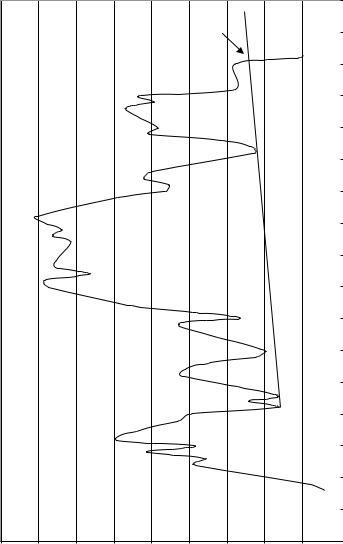
Sell!
Right shoulder
Head
Neckline
Left shoulder
96 |
95 |
94 |
93 |
92 |
91 |
90 |
89 |
88 |
|
|
|
|
|
Price |
|
|
|
|
7/16/2009 |
|
|
|
|
||
|
7/11/2009 |
|
|
|
7/6/2009 |
|
|
|
7/1/2009 |
|
|
|
6/26/2009 |
|
|
|
6/21/2009 |
|
|
|
6/16/2009 |
|
|
|
6/11/2009 |
SPY.for |
|
|
6/6/2009 |
||
|
|
||
|
6/1/2009 |
pattern |
|
|
5/27/2009 |
||
|
5/22/2009 |
shoulder- |
|
|
|
||
|
5/17/2009 |
-and |
|
|
5/12/2009 |
headthe |
|
|
|
||
|
5/7/2009 |
of |
|
|
5/2/2009 |
Example |
|
|
|
||
|
4/27/2009 |
10.5 |
|
|
4/22/2009 |
||
|
FIGURE |
||
|
|||
87 |
|||
115

116 |
TRADING STRATEGIES |
to the noise present in a training data sample and as a result have poor forecasting ability. Lo et al. (2000) and Omrane & Van Oppens (2004) demonstrate potential profitability of some complex geometric patterns. However, these profits may be too small for covering transaction costs.
SUMMARY
&The general picture of TA profitability is mixed. Careful statistical analysis demonstrates that simple TA strategies might be profitable in equities and in FX until the 1980s and 1990s, respectively.
&Diversification across various TA strategies and/or instruments used within the same (or similar) TA strategies may offer new opportunities for profitable trading.
&TA strategies may be a useful complimentary tool along with fundamental analysis.
&A simple taxonomy of TA strategies includes trend strategies (filter rules, moving-averages rules, and channel breakouts), momentum and oscillator strategies (MACD, RSI), and complex geometric patterns (head-and-shoulder, tops, bottoms, triangles, and others).

Financial Markets and Trading: An Introduction to
Market Microstructure and Trading Strategies by Anatoly B. Schmidt Copyright © 2011 Anatoly B. Schmidt
CHAPTER 11
Arbitrage Trading Strategies
According to the Law of One Price, equivalent assets (i.e., assets with the same payoff) must have the same price (see, e.g., Bodie & Merton 1998).
In competitive markets, the price of an asset must be the same worldwide providing that it is expressed in the same currency, and the transportation and transaction costs can be neglected. Violation of the Law of One Price leads to arbitrage, which is risk-free profiteering by buying an asset in a cheaper market and immediately selling it in a more expensive market.
In FX, a typical example of arbitrage is so-called triangle arbitrage. It appears in case of imbalance among three related currency pairs. Namely, exchange rates for three currencies X, Y, and Z generally satisfy the condition
ðX=YÞ ðZ=XÞ ðY=ZÞ ¼ 1 |
ð11:1Þ |
An arbitrage opportunity appears if (11.1) is violated. For example, if the product (EUR/JPY) (USD/EUR) is smaller than USD/JPY, one can buy JPY with USD, then buy EUR with JPY, and finally, make profits by buying USD for EUR.1
Arbitrage can continue only for a limited time until mispricing is eliminated due to increased demand and finite supply of a cheaper asset.2 Such a clear-cut (deterministic) opportunity, which guarantees a riskless gain, is sometimes called pure arbitrage (Bondarenko 2003). Deterministic arbitrage should be discerned from statistical arbitrage, which is based on statistical deviations of asset prices from their expected values and may incur losses (Jarrow et al. 2005). Note that practitioners use this term for denoting a specific trading strategy (see the next section).
Many arbitrage trading strategies are based on hedging the risk of financial losses by combining long and short positions in the same portfolio. An ultimate long/short hedging yields a market-neutral portfolio, in which risks from having long and short positions compensate each other.
117

118 |
TRADING STRATEGIES |
Market-neutral strategy can be described in terms of the CAPM. Indeed, since market-neutral strategy is supposed to completely eliminate market risk, the parameter bi (8.22) for the market-neutral portfolio equals zero.
As a simple example of market-neutral strategy, consider two companies within the same industry, A and B, one of which, say A, often yields higher returns. A simple investing approach might be buying shares A and neglecting shares B. A more sophisticated strategy named pair trading may involve simultaneously buying shares A and short selling shares B. Obviously, if the entire sector rises, this strategy does not bring as much money as simply buying shares A. However, if the entire market falls, it is expected that shares B will have higher losses than shares A. Then, profit from short selling shares B would compensate for the loss resulting from buying shares A. One possible problem with such thinking is that the persistent inferiority of company B in respect to A implies that B may be out of business after some time. Generally, pair trading is based on the idea of mean reversion (Vidyamurthy 2004). Namely, it is expected that the divergence in returns of similar companies A and B is a temporary effect due to market inefficiency, which is eliminated over some time. Pair trading strategy is then opposite to what we just described above. Namely, one should buy shares B and sell shares A.
Not all arbitrage trading strategies are market-neutral: The extent of long/short hedging is often determined by the asset fund manager’s discretion. The hedge fund industry has been using a taxonomy that includes not only strategy type but also instruments and geographic investment zones (Stefanini 2006; Khandani & Lo 2007).
This chapter continues with an overview of the major hedging strategies. Then, I focus on market-neutral pair trading, which has a straightforward formulation in terms of the econometric theory. Finally, recent studies of arbitrage risks are discussed.
H E D G I N G S T R A T E G I E S
Long/short hedging strategies are widely used by financial institutions, most notably by the hedge funds. Detailed specifics of these trading strategies are not widely advertised for the obvious reason: The more investors target the same market inefficiency, the faster it is wiped out. Still, general directions in the long/short hedging are well publicized (see, e.g., Stefanini 2006) and are outlined next.
Let’s start with equity hedge. Sometimes, one of two positions (e.g., the long one) is a stock index future while the other (short) one consists
Arbitrage Trading Strategies |
119 |
of all stocks that constitute this index (so-called index arbitrage). Pair trading and its special case, ADR arbitrage, also fit in this category. American depositary receipts (ADR) are securities that represent shares of non-U.S. companies traded in U.S. markets. Variations in market liquidity, trading volumes, and exchange rates may create discrepancies between prices of ADR and their underlying shares. Equity hedge may not be exactly the market-neutral one. Moreover, the ratio between long and short equity positions may be chosen depending on the market conditions. In recent years, so-called 130/30 (or more generally 1X0/X0, where X ¼ 2 5) mutual funds have gained popularity. These funds have 130 percent of their capital in long positions, 30 percent of which is funded by short positions. Sometimes, these portfolios are named long/ short funds. On the other hand, portfolios with dedicated short bias always have more short positions than the long ones.
Equity market-neutral strategy and statistical arbitrage. According to Khandani & Lo (2007), practitioners often use the term statistical arbitrage for describing the most challenging trading style: ‘‘highly technical short-term mean-reversion strategies involving large numbers of securities (hundreds to thousands, depending on the amount of risk capital), very short holding periods (measured in days to seconds), and substantial computational, trading, and IT infrastructure.’’ Equity market-neutral strategy is a less demanding approach that may involve lower frequency of trading and fewer securities. Economic parameters also may be incorporated into predicting models derived under the umbrella of mar- ket-neutral strategies.
Convertible arbitrage. Convertible bonds are bonds that can be converted into shares of the same company. Convertible bonds often decline less in a falling market than shares of the same company do. Hence, the idea of the convertible arbitrage may be buying convertible bonds and short selling the underlying stocks.
Fixed-income arbitrage. This strategy implies taking long and short positions in different fixed-income securities. Using analysis of correlations between different securities, one can buy those securities that seem to become underpriced and sell short those that look overpriced. One example is issuance-driven arbitrage, for example, on-the-run versus off-the-run U.S. Treasury bonds. Newly issued (on-the-run) Treasuries usually have yields lower than older off- the-run Treasuries but both yields are expected to converge with time. A more generic yield curve arbitrage is based on anomalies in

120 |
TRADING STRATEGIES |
dependence of bond yield on maturity. Other opportunities may appear in comparison of yields for Treasuries, corporate bonds, and municipal bonds.
Mortgage-backed securities (MBS) arbitrage. MBS is actually a form of fixed income with a prepayment option. Namely, mortgage borrowers can prepay their loans fully or partially prior to the mortgage term, which increases the uncertainty of the MBS value. While the MBS arbitrage is similar to the general fixed-income arbitrage, there are so many different MBS that this makes them a separate field of arbitrage expertise.
The strategies listed above can be combined into the family of relative value arbitrage. Another group of arbitrage strategies is called event-driven arbitrage. A typical example here is merger arbitrage (also called risk arbitrage). This form of arbitrage involves buying shares of a company that is expected to be bought and short selling the shares of the acquirer. The rationale behind this strategy is that businesses are usually acquired at a premium, which sends down the stock prices of acquiring companies. Another event-driven arbitrage strategy focuses on financially distressed companies. Their securities are sometimes sold below their fair values as a result of market overreaction to the news of distress.
Multi-strategy hedge funds use a synthetic approach that utilizes several hedging strategies and different securities. Looking for the arbitrage opportunities across the board is technically more challenging yet potentially rewarding. Global macro hedge funds apply their multiple strategies to instruments traded worldwide.
Stefanini (2006) offers a general review of historical performance of different arbitrage strategies. Khandani & Lo (2007) and Avellaneda & Lee (2010) find that performance of statistical arbitrage has generally degraded since 2002.
P A I R T R A D I N G
The general idea behind pair trading was introduced in the introduction to this chapter. Arbitrage Pricing Theory (APT) provides some theoretical background to this trading strategy (see, e.g., Grinold & Kahn 2000). The CAPM equation (8.23) implies that return on a risky asset is determined by a single non-diversifiable risk factor, namely by the risk associated with the entire market. APT offers a generic extension of CAPM into the multifactor paradigm. Namely, APT states that the return for an asset i at every time
Arbitrage Trading Strategies |
121 |
period is a weighed sum of the risk factor contributions fj(t) (j ¼ 1, |
. . . , K) |
plus an asset-specific random shock ei(t): |
|
RiðtÞ ¼ ai þ bi1f 1 þ bi2f 2 þ . . . þ biKf K þ eiðtÞ |
ð11:2Þ |
In (11.2), bij are the factor weights (betas). It is assumed that the expectations of all factor values and for the asset-specific innovations are zero:
E½f 1ðtÞ& ¼ . . . ¼ E½f KðtÞ& ¼ E½eiðtÞ& ¼ 0 |
ð11:3Þ |
Also, the risk factors of the asset-specific innovations are independent and uncorrelated:
Cov½f jðtÞ; |
f jðt0Þ& ¼ Cov½eiðtÞ; eiðt0Þ& ¼ 0; t ¼6 t0; |
Cov½f jðtÞ; |
ð11:4Þ |
eiðtÞ& ¼ 0 |
Then, APT states that there exist such K þ 1 constants l0, l1, . . . lK that
E½RiðtÞ& ¼ l0 þ bi1l1 þ . . . þ biKlK |
ð11:5Þ |
In (11.5), l0 has the sense of the risk-free asset return, and lj is called the risk premium for the jth risk factor. APT implies that similar companies have the same risk premiums and any deviation of returns from (11.5) is a mispricing, which yields arbitrage opportunities. For example, shares of an underpriced company should be bought while shares of an overpriced company should be shorted. Alas, APT does not contain a recipe for defining risk factors. These factors can be chosen among multiple fundamental and technical parameters. APT turns out to be more accurate for portfolios rather than for individual stocks. Hence, as Grinold & Kahn (2000) note, ‘‘APT is an art, not a science.’’
APT offers a valuable rationale for pursuing long/short trading strategies. Yet, it should be noted that buying underpriced and selling overpriced (in respect to the APT benchmark) securities in equal cash amounts does not guarantee market neutrality of the resulting portfolio. Truly market-neutral strategies do not need outside benchmarks; they employ relative mispricing, which can be recovered with the cointegration analysis.
C o i n t e g r a t i o n a n d C a u s a l i t y
Cointegration is an effective statistical technique developed by Engle and Granger for an analysis of common trends in multivariate time series (see, e.g., Hamilton 1994 and Alexander 2001). One might think that the