FinMarketsTrading

Financial Markets and Trading: An Introduction to

Market Microstructure and Trading Strategies by Anatoly B. Schmidt Copyright © 2011 Anatoly B. Schmidt

PART

Three

Trading Strategies

instruments. Timmerman (2006) concludes that simple forecasting schemes, such as equal-weighting of various strategies, are difficult to beat. For example, one popular approach is using multiple time frames (Kaufman 2005). Several trading strategies can be used simultaneously for the same asset. Hsu & Kuan (2005) have shown that trading strategies based on several simple technical rules can be profitable even if the standalone rules do not make money. Namely, Hsu & Kuan (2005) considered three strategies along with several technical rules including but not limited to moving averages and channel break-outs. One of these strategies, the learning strategy, is based on the periodic switching of investments to the best performing rule within a given class of rules. Another one, the voting strategy, assigns one vote to each rule within a given rule class. There are two choices: long positions and short positions. If most votes point at, say, a long position, this position is initiated. Finally, the position-changing strategy expands the voting strategy to fractional long/short allocation according to the ratio of long/short votes.

A promising approach has been offered by Okunev & White (2002). They tested three TA strategies for a portfolio consisting of up to seven currency pairs and found that this diversified portfolio outperformed returns for single currency pairs. Schulmeister (2009) performed simultaneous back-testing of 2,265 trading strategies for EUR/USD daily rates. This produced positive average yearly returns in 1999 through 2006.

Another option is to diversify portfolio assets rather than trading strategies. Wilcox and Crittenden (2005) applied long trend strategies to more than 24,000 securities for a period spanning 22 years, which significantly outperformed the buy-and-hold strategy for the S&P 500. Obviously, diversification has practical limits in partitioning a given investment capital among multiple strategies/instruments. Also, if transaction costs depend on the number of trades, maintaining a highly diversified dynamic portfolio may become prohibitively expensive. Still, these examples demonstrate that diversification may provide rich opportunities for implementing profitable TA strategies.

Recently, Neely et al. (2010) suggested mixing the trend strategies with an economic-variable model. This, too, may be a promising approach as the fundamental values improve in the end of recessions when prices are still depressed. On the other hand, the trend models are more sensitive to the beginning of recessions since the economic variables are generally updated quarterly. Hence, TA may be useful not only per se but also in combination with the fundamental value analysis.

The classical TA operates with daily market closing prices. Closing (and opening) of equity markets has an obvious meaning. However, it is less

definitive in FX that operates around the clock five days a week. With proliferation of day trading in recent years, numerous attempts to apply classical TA strategies to intraday price dynamics have been made.4

A generic notion of a bar is used in TA. Bar is usually defined with the time interval (e.g., daily bar or 10-minute bar). Sometimes equal-volume bars are used. Their size is determined with some trading volume typical for a given asset. Equal-volume bars have a shorter time duration within active trading hours (e.g., right after market opening) and a longer time duration during passive hours (e.g., around lunch time). Other major bar parameters include opening price, closing price, minimum price, and maximum price. In some strategies, such bar parameters as average price or volume-weighed average price may be used. Unless specified otherwise, we shall imply bar closing price while using the term price.

One common rule in the formulation of any trading strategies is to avoid look-ahead bias.5 Namely, trading rules should be expressed only in terms of lagged values. Indeed, while back-testing of trading strategies can be expanded into models defined in terms of present values, it is impossible to implement. In the following sections, I provide an overview of the primary strategies used in TA: trend strategies, momentum and oscillator strategies, as well as more complex patterns.

T R E N D S T R A T E G I E S

Trend strategies can be defined with the famous slogan, Buy low, sell high. The question is how low is low and how high is high? In other words, defining the market entry and market exit points remain a real challenge.

F i l t e r R u l e s

According to the simple filter rule (sometimes dubbed as the naive trading rule), one should buy/sell at the next opening if the last closing price Pk is higher/lower than the former closing price Pk 1 by a certain threshold d > 0 (usually chosen as higher than the asset daily volatility):

Buy: Pk=Pk 1 > 1 þ d

ð10:1Þ

Sell: Pk=Pk 1 < 1 d

The na€ıve strategy is sometimes used as a benchmark for comparative testing of other trading strategies (Dunis et al. 2003). In a more generic

approach, the highest/lowest closing prices for a given past period of length n are used for the trading decision (Taylor 2005). Namely,

Buy: Pk=Mk > 1 þ d

ð10:2Þ

Sell: Pk=mk < 1 d

where

Recent studies show that several filter rules (in terms of d and s) might be profitable in FX (but not in equities) until the 1980s, but this is not the case anymore, particularly if realistic transaction costs are accounted for (Park & Irwin 2007; Menkhoff & Taylor 2007). Still, filter rules offer great flexibility in formulating new strategies that may be worthy of further exploration. For example, Cooper (1999) suggested using prices and trading volumes at two (weekly) lagged periods for deriving buy/sell signals and demonstrated that increasing-volume stocks have weaker reversals (i.e., more pronounced trends), which leads to returns higher than those obtained from the buy-and-hold strategy.

M o v i n g - A v e r a g e R u l e s

Adding lagged periods in determining trends brings us to the moving averages techniques, which were already used in forecasting volatility (see Chapter 7). In the moving-average strategy, two moving averages (the short one and the long one) are compared to make a trading decision.

Let’s denote SMA over n lagged periods at time t with sma(Pt, n):

and consider the relative difference between the short-term (fast) sma(Pt, S) and the long-term (slow) sma(Pt, L):

The moving-average strategy generates the following trading signals:

Buy: rt > d

ð10:6Þ

Sell: rt < d

Simple moving averages may be replaced with the exponential moving average (EMA)

As was indicated in Chapter 7, the smoothing coefficient b has the following relation to the number of lagged periods:

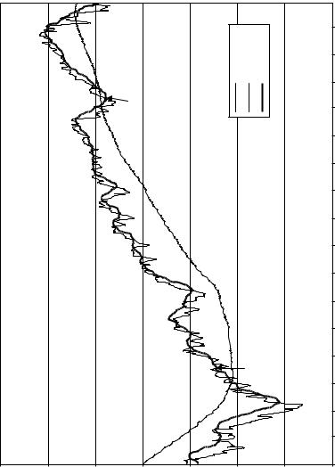
The value of P0 is usually chosen to be equal to the sma(Pt, n) for a short initial period. Typical ratios L/S in the known literature vary in the range 420. An example of the moving-average strategy (and the challenges it faces) is given for SPY in Figure 10.1. While the buy signal in April 2009 can be noticed in a rather wide range of d (i.e., there is a pronounced trend), low d can generate a Sell signal in February 2010, which probably could be ignored.

Several adaptive moving-average strategies have been proposed by practitioners to account for the potentially non-stationary nature of price dynamics (Kaufman 2005). The idea here is to treat lags S and L as variables that depend on price variations. An example of such an approach is Chande’s Variable Index Dynamic Average (VIDYA), in which exponential smoothing depends on price volatility:

In (10.9), b is the smoothing coefficient and k ¼ stdev(Pt, S)/stdev(Pt, L) is the relative volatility calculated for S recent lags and a longer past period L.

C h a n n e l B r e a k o u t s

A channel (or band) is an area that surrounds a trend line within which price movement does not indicate formation of a new trend. The upper and bottom walls of channels have a sense of resistance and support. Trading strategies based on the channel breakouts are popular among practitioners and in academy (Park & Irwin 2007). One way to formulate the trading rules with channel breakouts is as follows (Taylor 2005). If a trader has long position at time t, the sell signal is generated when

Here, B is the channel bandwidth and the values of mt and Mt are defined in (10.3). If a trader has a short position at time t, a buy signal is generated when

Finally, if a trader is neutral at time t, the conditions (10.10) and (10.11) are signals for acquiring short and long positions, respectively. A more risky strategy may use a buy signal when

In the Bollinger bands, which are popular among practitioners, the trend line is defined with the price SMA (or EMA), and the bandwidth is determined by the asset volatility

The parameters k and L in (10.14) are often chosen to be equal to 2 and 20, respectively.

M O M E N T U M A N D O S C I L L A T O R S T R A T E G I E S

In TA, the term momentum is used for describing the rate of price change. In particular, K-day momentum at day t equals

Momentum smoothes price and can be used either for generating trading signals or as a trend indicator. For example, a simple momentum rule may be a buy/sell signal when momentum switches from a negative/positive value to a positive/negative one.

Sometimes, momentum is referred to as the difference between current price and its moving average (e.g., EMA).

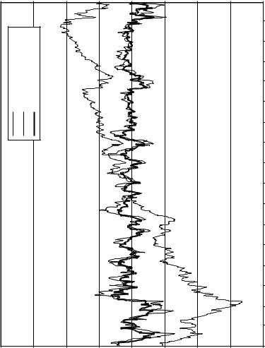
Momentum (10.16) leads to further price smoothing (see Figure 10.2).