

Учебный год 22-23 / Firms, Contracts, and Financial Structure
.pdf40 |
I. UNDERSTANDING FIRMS |
The Second-Best Choice of Investments.
Now consider the second-best incomplete contracting world, where the parties choose their investments noncooperatively at date 0. Suppose that the ownership structure is such that M1 owns the set of assets A and M2 owns the set of assets B. Then from (2.4) and (2.5) M1's and M2's payoffs, net of investment costs, are given by(2.10)
(2.11)
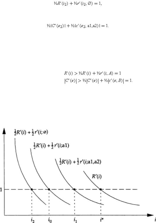
Differentiating (2.10) with respect to i and (2.11) with respect to e yields the following necessary and sufficient conditions for a (Nash) equilibrium:(2.12)
(2.13)
For future reference, it is useful to write out (2.12) and (2.13) for the three ‘leading’ ownership structures.
Non-Integration.
The equilibrium is characterized by(2.14)
(2.15)
(Here the subscript 0 stands for no integration.)
Type 1 Integration.
The equilibrium is characterized by(2.16)
(2.17)
(Here the subscript 1 stands for type 1 integration.)
2. THE PROPERTY RIGHTS APPROACH |
41 |
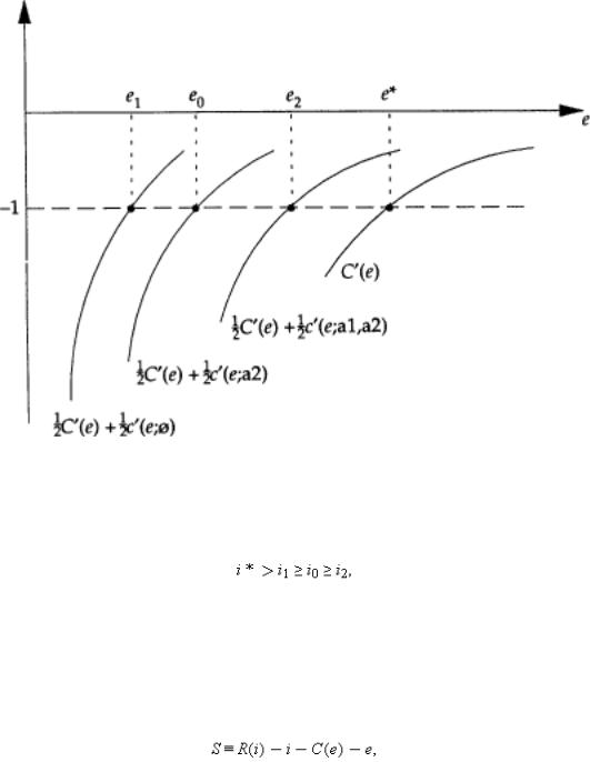
Type 2 Integration.
The equilibrium is characterized by(2.18)
(2.19)
(Here the subscript 2 stands for type 2 integration.)
Under assumptions (2.2) and (2.3), (2.12) and (2.13) yield the following result about all second-best outcomes.
PROPOSITION 1. |
Under any ownership structure, there is underinvestment in relationship-specific investments. |
|
That is, the investment choices in (2.12) and (2.13) satisfy i<i*, e<e*. |
Proof. |
Suppose i, e satisfy (2.12) and (2.13). Then, by (2.2) and (2.3), |
The result follows since R″<0, C″>0.□
The intuition for the underinvestment result is as follows. If M1 invests a little more, this increases the gains from trade by R′(i). However, M1's payoff increases only by 1/2R′(i)+1/2r′(i;A)<R′(i); the remaining gains go to M2. Being selfinterested, M1 does not take M2's payoffs into account and hence invests too little. A similar argument applies to M2.44
Fig. 2.2
44 Not all models of ownership yield underinvestment. For example, in Grossman and Hart (1986), overinvestment is possible as well as underinvestment. This is because (2.2) and (2.3) do not hold in the Grossman–Hart model.
42 |
I. UNDERSTANDING FIRMS |
Fig. 2.3
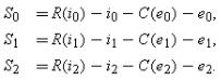
The first-best outcome, and the second-best outcomes under non-integration and type 1 and type 2 integration, are illustrated in Figures 2.2 and 2.3.45 It is clear from these figures what the effects of integration are. Relative to nonintegration, type 1 integration raises M1's investment, but lowers M2's. Relative to non-integration, type 2 integration raises M2's investment, but lowers M1's. That is,(2.20)
(2.21)
For future reference, note that efficient ex post bargaining implies that the total surplus from the relationship under any ownership structure is given by(2.22)
where i and e satisfy (2.12) and (2.13).46
45 |
Proposition 1 has been derived under the assumptions that the ex post surplus when M1 and M2 trade, given by T |
(i, e )≡R (i )−C (e |
), is separable in i and e ; i.e. (∂2 /∂i |
||
|
∂e )T (i, e )=0. Proposition 1 can be shown to generalize to the case (∂2 /∂i ∂e |
)T (i, |
e )≥0 (i.e., i and e |
are complements); see Hart and Moore (1990). |
|
46 |
In this model, ownership structure matters because it affects the no-trade payoffs r |
and c |
(more particularly, the marginal payoffs r |
′ and c ′). Not all bargaining solutions |
|
have the property that the equilibrium outcome depends on the no-trade payoffs. For example, in a bargaining game with outside options, the equilibrium division of surplus is independent of the no-trade payoffs (that is, the outside options) within a certain range (see, e.g., Osborne and Rubinstein 1990). However, what is important for the analysis of ownership is that the no-trade payoffs sometimes matter, not that they always matter. With a reasonable amount of ex ante uncertainty about investment returns, the no-trade payoffs will affect the equilibrium division of surplus with positive probability even in a bargaining game with outside options. Thus, the main ideas of the analysis of ownership will continue to be relevant.
2. THE PROPERTY RIGHTS APPROACH |
43 |
Ex Ante Division of Surplus
Little has been said so far about how the surplus S is divided under a particular ownership structure. Equations (2.10) and (2.11) correspond to the ex post division, but, given that lump-sum transfers are possible at date 0, the ex ante division may be different. I shall suppose that M1 has many potential trading partners at date 0, but M1 is unique. Then M2 will receive her reservation payoff at date 0, V say, and M1 will get all the gains from the relationship, S−V.47 Nothing depends on this assumption about relative bargaining power, however. In fact, as will be seen, the size of V plays no role in the analysis of optimal ownership structure (as long as (S−V) exceeds M1's date 0 reservation payoff; I assume this in what follows).
The Choice of Ownership Structure
The last step is to determine which ownership structure is best. This is straightforward. Simply compute the total surplus from the various arrangements. (The division of surplus is unimportant since this can always be adjusted using lump-sum transfers at date 0.) In other words, compare the following:(2.23)
47More generally, the ex ante division of surplus will be determined by the degree of competition in the market for alternative ‘M1s’ and ‘M2s’ at date 0, that is, by how many potential trading partners M1 has and how many potential trading partners M2 has. Note that relative bargaining power at date 0 may be very different from relative
bargaining power at date 1 since relationship-specific investments have not yet been made at date 0. Williamson (1985) has referred to this as ‘the fundamental transformation’.

44 |
I. UNDERSTANDING FIRMS |
The theory predicts that the ownership structure that yields the highest value of S will be chosen in equilibrium. For example, if at the starting point of their relationship M1 owns a1 and M2 owns a2, and S1>Max(S0, S2), then M1 will buy a2 from M2 at some price that will make them both better off. (In fact, given the assumptions about relative bargaining power, the price will be such that M2's final payoff is V.)
Analysis of the Optimal Ownership Structure
I now consider in greater detail what forces favour one ownership structure over another. Before I start, it is worth making a simple observation. As is clear from (2.12)–(2.13), any change in ownership structure that increases r′(i;·) (resp., increases |c′(e;·)|) without decreasing |c′(e;·)| (resp., decreasing r′(i;·)), or more generally that increases i or e without decreasing the other, is good. The reason is that, since both parties (always) underinvest (see Proposition 1), such a change moves the parties closer to the first-best and so total surplus given by R(i)−i−C(e)−e rises.
It is useful to introduce some definitions.
DEFINITION 1. M1's investment decision will be said to be inelastic in the range 1/2≤ρ≤1 if the solution to MaxiρR(i)−i is independent of ρ in this range. Similarly, M2's investment decision will be said to be inelastic in the range 1/2≤σ≤1 if the solution to MineσC(e)+e is independent of σ in this range.48
DEFINITION 2. M1's investment will be said to become relatively unproductive if R(i) is replaced by θR(i)+(1−θ)i, and r(i;A) is replaced by θr(i;A)+(1−θ)i for all A=a1, (a1, a2) or Ø, where θ>0 is small. M2's investment will be said to become relatively unproductive if C(e) is replaced by θC(e)−(1−θ)e, and c(e;B) is replaced by θc(e;B)−(1−θ)e for all B=a2, (a1, a2) or Ø, where θ>0 is small.
DEFINITION 3. Assets a1 and a2 are independent if r′(i;a1, a2)≡r′(i;a1) and c′(e;a1, a2)≡c′(e;a2).
48 For M1's investment decision to be inelastic, it must be the case that, for some |
for |
|
be inelastic, it must be the case that, for some |
for 0<e <ê and |C ′(e )|<1 for |
|
everywhere is relaxed. |
|
|
for ; and for M2's investment decision to
. In Definition 1, therefore, the assumption that R ″ and C ″ exist
|
2. THE PROPERTY RIGHTS APPROACH |
45 |
DEFINITION 4. |
Assets a1 and a2 are strictly complementary if either r′(i;a1)≡r′(i;Ø) or c′(e;a2)≡c′(e;Ø). |
|
DEFINITION 5. |
M1's human capital (resp., M2's human capital) is essential if c′(e;a1, a2)≡c′(e;Ø) (resp., |
r′(i;a1, |
|
a2)≡r′(i;Ø)). |
|
These definitions are intuitive. The first one guarantees that M1 (resp., M2) will choose the same level of i,î say, (resp., the same level of e,ê say) in any one of the ownership structures with 50: 50 bargaining.
In the second definition, the net social return from M1's (resp., M2's) investment, R(i)−i, becomes θ(R(i)−i) (resp., C(e)+e becomes θ(C(e)+e)), which is small when θ is small. In other words M1's (resp., M2's) investment becomes unimportant relative to M2's (resp., M1's).
The third definition says that a1 and a2 are independent if access to a2 will not increase M1's marginal return from investment given that he already has access to a1; and if access to a1 will not increase M2's marginal return from investment given that she already has access to a2.
The fourth definition says that a1 and a2 are strictly complementary either if access to a1 alone has no effect on M1's marginal return from investment (M1 needs a2 as well), or if access to a2 alone has no effect on M2's marginal return from investment (M2 needs a1 as well).
Finally, the fifth definition says that one party's human capital is essential if the other party's marginal return from investment is not enhanced by the presence of the assets a1 and a2 in the absence of the first party's human capital.
Proposition 2 makes use of the above definitions.
PROPOSITION2.(A) If M2's investment decision (resp., M1's investment decision) is inelastic, then type 1 integration
|
(resp., type 2 integration) is optimal. |
(B) |
Suppose M2's investment (resp. M1's investment) becomes relatively unproductive, and r′(i;a1, |
|
a2)>r′(i;a1) for all i (resp. |c′(e;a1, a2)|>|c′(e;a2)| for all e). Then, for θ small enough, type 1 |
|
integration (resp., type 2 integration) is optimal. |
(C) |
If assets a1 and a2 are independent, then non-integration is optimal. |
46 |
I. UNDERSTANDING FIRMS |
(D) |
If assets a1 and a2 are strictly complementary, then some form of integration is optimal. |
(E) |
If M1's (resp., M2's) human capital is essential, then type 1 (resp., type 2) integration is optimal. |
(F) |
If both M1's human capital and M2's human capital are essential, then all ownership structures |
|
are equally good. |
Proof. (A) |
Suppose M2's investment decision is inelastic. Then (2.3) and (2.13) imply that M2 sets e=ê under |
|
all ownership structures. Thus, it is best to give all the control rights to M1. Conversely, if M1's |
|
investment decision is inelastic, it is best to give all the control rights to M2. |
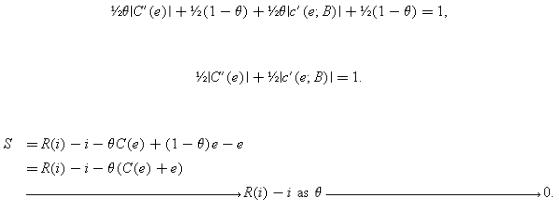
(B) |
Suppose that M2's investment is relatively unproductive. Then M2's first-order condition under |
|
any ownership structure becomes (see (2.13)): |
|
which simplifies to |
|
In other words, M2's investment decision is independent of θ. However, net surplus, given by |
|
Thus, for θ small, what matters is M1's investment decision. Hence it is optimal to give all the |
|
control rights to M1. The same argument shows that M2 should have all the control rights if M1's |
|
investment is relatively unproductive. |
(C) |
Note that, by the definition of independence, the solutions to (2.14) and (2.16) are the same; that |
|
is, i1=i0. Since e1≤e0, non-integration dominates type 1 integration. Also, the solutions to (2.15) and |
|
(2.19) are the same; that is, e2=e0. Since i2≤i0, non-integration dominates type 2 integration. |
(D) |
Suppose first that r′(i;a1)≡r′(i;Ø). Then the solutions to (2.14) and (2.18) are the same; that is, i0=i2. |
|
Since e0≤e2, type 2 integration dominates non-integration. The same argument shows that, if |
|
c′(e;a2)≡c′(e;Ø), type 1 integration dominates non-integration. |
(E) |
Note that, if M1's human capital is essential, then the solutions to (2.15), (2.17), and (2.19) are all |
|
the same; that is, |
|
2. THE PROPERTY RIGHTS APPROACH |
47 |
|
e0=e1=e2. Since i1≥i0≥i2, type 1 integration is optimal. The same argument shows that, if M2's |
|
|
human capital is essential, type 2 integration is optimal. |
|
(F) |
This follows from the fact that, if M1 and M2's human capital are both essential, the solutions to |
|
|
(2.14), (2.16), and (2.18) are all the same and so are the solutions to (2.15), (2.17), and (2.19); that |
|
|
is, i0=i1=i2 and e0=e1=e2. Thus, organizational form is irrelevant. □ |
|
Most of Proposition 2 is very intuitive. Part (A) says that there is no point giving ownership rights to a party whose investment decision is not responsive to incentives. Part (B) says that there is no point giving ownership rights to a party whose investment is unimportant. Parts (C)–(F) are a little more striking, and it is worth saying a bit more about them.
To understand (C), start with non-integration and consider transferring control of a2 from M2 to M1. This has no effect on M1's marginal return from investment in the event that the parties fail to reach agreement since a1 is no more useful with a2 than without; but transferring control to M1 may have a significantly negative effect on M2's marginal investment return, since without a2 M2 may be able to achieve very little. Thus, the effect of the control transfer is to keep i constant but reduce e, which reduces total surplus. A similar logic applies if we transfer control of a1 from M1 to M2: e stays constant, but i may fall significantly. Thus, when the assets are independent, both forms of integration are dominated by non-integration.
Consider next (D). Start with non-integration. If a1 and a2 are strictly complementary, then transferring control of a2 from M2 to M1 weakly increases M1's marginal return from investment (his return from investment absent an agreement with M2 rises), but it has no effect on M2's marginal return. The reason is that a2 is useless without a1 and so giving up a2 does not change M2's return absent an agreement with M1. Thus, moving from non-integration to integration yields benefits but no costs. A similar logic applies as one moves from non-integration to type 2 integration; hence type 2 integration also is superior to non-integration. Thus, when the assets are strictly complementary, some form of integration is better than non-integration, but without further information (about, say, the importance of M1's investment
48 |
I. UNDERSTANDING FIRMS |
relative to M2's) it is not possible to rank type 1 integration against type 2 integration.
To understand (E), note that, if M1's human capital is essential, then transferring assets from M2 to M1 has no effect on M2's investment incentives, since M2's no-trade payoff does not depend on the assets she has in the absence of M1's human capital (at the margin). Thus, there is no cost of the control transfer. However, there may be a benefit, since if M1 has all the assets this is likely to increase his incentive to invest.
Note that (B) and (E) together can be summarized as saying that a party with an important investment or important human capital should have ownership rights.
Finally, (F) says that, if both M1 and M2 have essential human capital, then ownership structure does not matter since neither party's investment will pay off in the absence of agreement with the other.
Two observations are worth making. First, the argument showing that complementary assets should be owned together also shows that joint ownership of an asset is suboptimal. Suppose a1 is owned by both M1 and M2. What this means is that if negotiations break down neither M1 nor M2 has access to a1 independently (since any asset usage must be agreed by both). However, such an arrangement is equivalent to dividing a1 in two and assigning one half to M1 and the other half to M2. Since it is clear that the two halves are strictly complementary, an argument similar to that in the proof of Proposition 2(D) tells us that such an outcome is dominated by one in which all of a1 is assigned to either M1 or M2. (This is true whoever is the owner of a2.)49
A caveat is important here. I have supposed that the investments i and e are embodied in M1 and M2's human capital, in the sense that M1 does not obtain the benefit of e unless he reaches agreement with M2, and M2 does not obtain the benefit of i unless she reaches agreement with M1. As will be seen in Chapter 3, if investments are embodied in physical assets rather than human assets, it is no longer clear that strictly complementary assets
49 This argument assumes that an asset cannot be used by two people independently. However, for some assets joint usage is possible. For example, a patent can be developed and marketed by two separate firms. In such a case, joint ownership may be optimal. See Aghion and Tirole (1994) and Tao and Wu (1994).
2. THE PROPERTY RIGHTS APPROACH |
49 |
should be owned by the same person (or that assets should not be jointly owned).50
Second, it should be noted that there is another ownership arrangement that has not been considered: ‘reverse’ nonintegration, in which M1 owns a2 and M2 owns a1. It is easy to rule this arrangement out, however. Since a1 is the primary asset M1 works with and a2 is the primary asset M2 works with, one would expect M1 to be more productive with a1 than with a2 and M2 to be more productive with a2 than with a1. In other words, one would expect r′(i;a2)—the marginal return on M1's investment if he has access only to a2—to be less than r′(i;a1), and |c′(e;a1)|—the marginal return on M2's investment if she has access only to a1—to be less than |c′(e;a2)|. It follows immediately from this that non-integration dominates this fourth ownership arrangement.51
3.Simple Things the Theory Can Tell Us About the World
To conclude this chapter, I would like to consider whether the theory's predictions match up with the actual organizational arrangements observed. Unfortunately, there has to date been no formal testing of the property rights approach, and so in what follows I do not attempt to go beyond what is impressionistic.
One very simple implication of the theory is that, ceteris paribus, a party is more likely to own an asset if he or she has an important investment decision (where the investment decision might represent figuring out how to make the asset more productive or looking after the asset). As an example of this, consider the fact
50It is also not clear that Proposition 2(D) generalizes to the case where contracts are partially, but not totally, incomplete, i.e. where long-term contracts have some role to play. The reason is that Proposition 2(D) depends on the idea that allocating a2 to M2, say, in the absence of a1 does not increase M2's marginal return if bargaining breaks down (since a2 is useless without a1), but does lower M1's marginal return. However, if a long-term contract is in place, then disagreement corresponds to sticking to the original contract. In this case, a2 may have value to M2 under the original contract, even if M2 does not own a1, and there may therefore be some gain from allocating a2 to M2.
51I have also ignored stochastic ownership structures, i.e. arrangements in which, say, M1 owns a2 with probability σ and M2 owns a2 with probability (1−σ). These are discussed further in Ch. 4.