

Учебный год 22-23 / Firms, Contracts, and Financial Structure
.pdf10 |
INTRODCUTION |
people, then no one of them may have an incentive to be active in exercising this power. It is then important that there exist automatic mechanisms that will achieve what those with power are unable or unwilling to do by themselves.
A leading example of dispersed power is the case of a public company with many, small shareholders. Shareholders cannot run the company themselves on a day-to-day basis and so they delegate power to a board of directors and to managers. This creates a free-rider problem: an individual shareholder does not have an incentive to monitor management, since the gains from improved management are enjoyed by all shareholders, whereas the costs are borne only by those who are active. Because of this free-rider problem, the managers of a public company have a fairly free hand to pursue their own goals: these might include empire-building or the enjoyment of perquisites.
Chapters 6 and 8 explore two ‘automatic’ mechanisms that can improve the performance of management: debt (in combination with bankruptcy) and take-overs. Debt imposes a hard budget constraint on managers. If a company has a significant amount of debt, management is faced with a simple choice: reduce slack—that is, cut back on empirebuilding and perquisites—or go bankrupt. If there is a significant chance that managers will lose their jobs in bankruptcy, they are likely to choose the first option.
Take-overs provide a potential way to overcome collective action problems among shareholders. If a company is badly managed, then there is an incentive for someone to acquire a large stake in the company, improve performance, and make a gain on the shares or votes purchased. The threat of such action can persuade management to act in the interest of shareholders.
I derive some implications of these views of debt and take-overs. Chapter 6 shows that the view of debt as a constraining mechanism can explain the types of debt a company issues (how senior the debt is, whether it can be postponed). Chapter 8 shows that the possibility of take-overs can explain why many companies bundle votes and dividend claims together—that is, why they adopt a one share–one vote rule. One share–one vote protects shareholder property rights in the sense that it maximizes the chance that a control contest will be won by a management team that provides high value for shareholders, rather than high private benefits for itself.
INTRODUCTION |
11 |
Of course, if a company takes on debt, then there is always the chance that it will go bankrupt. If contracting costs were zero, there would be no need for a formal bankruptcy procedure because every contract would specify what should happen if some party could not meet its debt obligations. In a world of incomplete contracts, however, there is a role for bankruptcy procedure. In Chapter 7 I argue that a bankruptcy procedure should have two main goals. The first is that a bankrupt company's assets should be placed in their highest-value use. The second is that bankruptcy should be accompanied by a loss of power for management, so as to ensure that management has the right incentive to avoid bankruptcy. Chapter 7 suggests a procedure that meets these goals, and at the same time avoids some of the inefficiencies of existing US and UK procedures.
5. An Omitted Topic: Public Ownership
The book is concerned with the optimal allocation of privately owned assets. A very important topic not considered concerns the optimal balance between public and private ownership. Which assets should be publicly owned and which should be privately owned? This issue has always been a central one in the economic and political debate, but it has attracted new attention in the last few years as major industries have been privatized in the West and the socialist regimes in Eastern Europe and the former Soviet Union have dissolved.
It is natural to analyse public choice versus private choice using the ideas of incomplete contracts and power. If contracting costs are zero, there is no difference between the optimal regulation of a private firm on the one hand, and nationalization or public ownership on the other. In both cases the government will write a ‘comprehensive’ contract with the firm or its managers that will anticipate all future contingencies. The contract will specify the manager's compensation scheme, how the price of the firm's output should change if costs fall, how the nature of the firm's product should change if there is a technological innovation or a shift in demand, etc.
In contrast, in a world of incomplete contracts, public and private ownership are different, since in one case the government
12 |
INTRODCUTION |
has residual control rights over the firm's assets, while in the other case a private owner does. The public–private case is not a simple extension of the pure private property rights model, however. At least two new questions arise. First, what is the government's objective function? Much existing work views the government as a monolith, but this is unsatisfactory since, even more than in the case of a corporation, the government represents a collection of agents with conflicting goals: civil servants, politicians, and the citizens themselves. Second, what ensures that the government respects an agreed-on allocation of property rights? The government, unlike a private agent, can always change its mind: it can nationalize assets it has privatized or privatize assets it has nationalized.
There is a small, but growing, literature that analyses public versus private ownership in incomplete contracting terms.9 However, much remains to be done. Developing a satisfactory theory, which deals among other things with the issue of the government's objective function and its commitment to property rights, is a challenging but fascinating task for future research.
9 |
See, in particular, Schmidt (1990), Shapiro and Willig (1990), Shleifer and Vishny (1994), and Boycko et al. (1995). |
|
Part I Understanding Firms
The first part of the book, Chapters 1–4, is concerned with the nature and extent of the firm, that is, with the determinants of the boundaries of firms in a market economy. Chapter 1 contains a discussion of existing theories of the firm, including the neoclassical, principal–agent, and transaction cost theories. While these theories have proved very useful for some purposes, I shall argue that they cannot by themselves explain the boundaries of firms (or the internal organization of firms). Chapters 2 and 3 describe the more recent incomplete contracting or ‘property rights’ approach, which can throw some light on firm boundaries. This theory can also explain the meaning and importance of asset ownership. Finally, Chapter 4 provides a discussion of the foundations of the incomplete contracting model used in Part I and, to some extent, throughout the book.
This page intentionally left blank
1 Established Theories of the Firm
This chapter discusses some of the ways in which economists have looked at firms. I begin with the neoclassical theory of the firm, the standard approach found in all textbooks. I then move on to the principal–agent and transaction cost theories.10
1. Neoclassical Theory
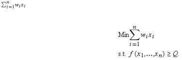
Neoclassical theory, which has been developed over the last one hundred years or so, views the firm mainly in technological terms. A single-product firm is represented by a production function which specifies the output level Q that is obtained when given levels of n inputs x1, . . . ,xn are chosen. It is supposed that the firm is run by a selfless manager, M, who chooses input and output levels to maximize profit. This in turn implies that the manager minimizes costs.
The simplest case is where M purchases the n inputs in a competitive market at given prices w1, . . . ,wn, so that his total costs are . Let Q=f(x1, . . . ,xn) denote the firm's production function. Then, given a target output level Q, M will minimize costs by solving the following problem:
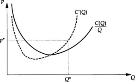
Solving this for every value of Q generates a total cost curve C(Q), from which can be deduced an average cost curve C(Q)/Q and a marginal cost curve C′(Q). The latter two curves are assumed to have the familiar shape indicated in Figure 1.1.
10 Readers may find it useful to consult some other recent accounts of the theory of the firm, e.g. Holmstrom and Tirole (1989), Milgrom and Roberts (1992), and Radner (1992).
16 |
I. UNDERSTANDING FIRMS |
Fig. 1.1
The second stage of M's problem is to decide what level of output to produce. Under the assumption that M is a perfect competitor in the output market and faces price p*, he maximizes p*Q−C(Q). This leads to the familiar equality between price and marginal cost, illustrated in Figure 1.1.
The U-shape of the average cost curve is justified as follows. There are some fixed costs of production (plant, machines, buildings) that must be incurred whatever the level of output. As output increases, variable costs increase, but fixed costs do not. Thus, there is a tendency for per-unit costs to fall. However, after a certain point further expansion becomes difficult because some inputs cannot be varied easily with the firm's scale. One of these is managerial talent. As output rises, the manager eventually becomes overloaded and his productivity falls. As a consequence, the firm's average cost begins to rise.11
How should one assess this theory of the firm? On the positive side, the theory is surely right to stress the role of technology in general, and returns to scale in particular, as important determinants of the size of firms (see e.g. Chandler 1990: 26–8). In addition, the theory has been very useful for analysing how the firm's optimal production choice varies with input and output prices, for understanding the aggregate behaviour of an industry, and for studying the consequences of strategic interaction between
11 For a more general account of the neoclassical theory of the firm, see Mas-Colell et al. (1995: ch. 5).
1. ESTABLISHED THEORIES OF THE FIRM |
17 |
firms once the assumption of perfect competition has been dropped (see e.g. Tirole 1988).
At the same time, the theory has several serious weaknesses. First, it completely ignores incentive problems within the firm. The firm is treated as a perfectly efficient ‘black box’, inside which everything operates perfectly smoothly and everybody does what they are told. Even a cursory glance at any actual firm suggests that this is unrealistic. Second, the theory has nothing to say about the internal organization of firms—their hierarchical structure, how decisions are delegated, who has authority. Third, and related, the theory does not satisfactorily pin down the bound-aries of the firm. Among other things, it is not clear why managerial talent is a fixed factor: why can't the managerial diseconomies that lie behind the upward-sloping portion of the average cost curve be avoided through the hiring of a second manager?
It is useful to dwell on this last point since it lies at the heart of the first part of this book. Neoclassical theory is as much a theory of division or plant size as of firm size. Consider Figure 1.1 again. Imagine two ‘firms’ with the same production function f and cost function C, each facing the output price p* (and both being perfect competitors). Neoclassical theory predicts that in equilibrium each firm produces Q*. But couldn't one just as well imagine a single large firm operating with each of the smaller firms as divisions, producing 2Q* altogether?
This line of reasoning suggests that it is not enough to argue that a firm will not expand because its manager has special skills and additional managers are inferior. The real issue is why it makes sense for the additional managers to be employed outside this firm, rather than within a division or subsidiary operated by this firm. In other words, given the original firm and a second firm employing an alternative manager, why doesn't the first firm expand—possibly laterally—by merging with the second firm?
To put it in stark terms (suggested originally by Coase 1937), neoclassical theory is consistent with there being one huge firm in the world, with every existing firm (General Electric, Exxon, Unilever, British Petroleum, . . . ) being a division of this firm. It is also consistent with every plant and division of an existing firm becoming a separate and independent firm. To distinguish between these possibilities, it is necessary to introduce factors not present in the neoclassical story.

18 |
I. UNDERSTANDING FIRMS |
2. The Agency View
As noted, neoclassical theory ignores all incentive problems within the firm. Over the last twenty years or so, a branch of the literature—principal–agent theory—has developed which tries to rectify this. I shall argue that principal–agent theory leads to a richer and more realistic portrayal of firms but that it leaves unresolved the basic issue of the determinants of firm boundaries.
A simple way to incorporate incentive considerations into the neoclassical model described above is to suppose that one of the inputs, input i say, has a quality that is endogenous, rather than exogenous. In particular, suppose that input i (a widget, say) is supplied by another (owner-managed) ‘firm’, and that the quality of this input, q, depends on the effort the supplying manager exerts, e, as well as on some randomness outside the manager's control, Î:
Here Î is assumed to be realized after the manager's choice of e.12
Assume that quality q is observable and verifiable—it might represent the fraction of widgets that are not defective—but that the purchasing manager does not observe the supplying manager's effort, nor does he observe Î.13 Assume also that the supplying manager dislikes high effort; represent this by a ‘cost of effort’ function H(e). Finally, suppose (for simplicity) that only one widget is required by the purchaser (xi=1), that this yields the purchaser a revenue of r(q), and that the supplying manager is risk-averse, while the purchasing manager is risk-neutral.14
If the purchaser could observe and verify e, he would offer the supplier a contract of the form: ‘I will pay you a fixed amount P* as long as you choose the effort level e*.’ Here e* is chosen to be
12Another version of the principal–agent problem assumes that Î is realized before the manager's choice of e ; see e.g. Laffont and Tirole (1993: ch. 1).
13The statement that q is observable and verifiable means that the parties can write an enforceable contract on the value of q.
14 Let the purchasing manager's utility function be Up (r (q )−P )=r (q )−P and the supplying manager's utility function be Us (P, e )=V (P )−H (e ), where V is concave, and P represents the payment made by the purchasing manager to the supplying manager. The principal–agent problem is interesting only if the supplying manager is riskaverse. Letting the purchasing manager be risk-neutral is a simplifying assumption.
1. ESTABLISHED THEORIES OF THE FIRM |
19 |
jointly efficient for the purchaser and the supplier and P* is determined so as to divide up the gains from trade between the two parties, according to the relative scarcity of potential purchasers and suppliers, relative bargaining power, etc.15
The advantage of the fixed payment P* is that it ensures optimal risk-sharing. The purchaser bears all the risk of Î realizations, which is efficient since he is risk-neutral and the supplier is risk-averse.
Unfortunately, when e is not observable to the purchaser, the above contract is not feasible, since it cannot be enforced. (The purchaser would not know if the supplier deviated from e=e*.) To put it another way, under the above contract, the supplier would set e=0 if she dislikes working. To get the supplier to exert effort, the purchaser must pay the supplier according to observed performance q, i.e. he must offer the supplier an incentive scheme P=P(q). In designing this incentive scheme, the two parties face the classic trade-off between optimal incentives and optimal risksharing. A ‘high-powered’ incentive scheme—that is, one where P′(q) is close to r′(q)—is good for supplier incentives since the supplier earns a large fraction of the gains from any increase in e; but it exposes the supplier to a great deal of risk. Conversely, a low-powered scheme protects the supplier from risk but gives her little incentive to work hard.16
There is now a vast literature that analyses the form of the optimal incentive scheme under the above circumstances. Moreover, the basic principal–agent problem described has been extended in a number of directions. Among other things, agency theorists have allowed for: repeated relationships, several agents, several principals, several dimensions of action for the agent, career concerns and reputation effects, and so on.17
As a result of all this work, a rich set of results about optimal
15 |
Given the utility functions described in n. 5, and assuming that the supplying manager receives an expected utility of U, it is easy to show that e * maximizes E [r (g |
|
|
(e,Î))]−V−1 (U +H (e )), and P *=V−1 (U +H (e *)), where E |
is the expectations operator. For details, see Hart and Holmstrom (1987). |
16 |
An optimal incentive scheme solves the following problem: Max |
E[r(g(e,Î))−P(g(e,Î))] |
e, P(•)
s.t. (1) eÎargmaxe′{E[V(P(g(e′,Î)))]−H(e′)},
(2)E[V(P(g(e,Î)))]−H(e)≥U.
For details, see Hart and Holmstrom (1987).
17 For surveys, see Hart and Holmstrom (1987) and Sappington (1991).