

Учебный год 22-23 / Firms, Contracts, and Financial Structure
.pdf130 |
II. UNDERSTANDING FINANCIAL STRUCTURE |
The above four assumptions, although strong, seem to be reasonable starting points for a study of a public company. The first captures the idea that investors are wealth-constrained. Note that this assumption effectively rules out renegotiation with creditors (because of free-rider problems; see Ch. 5, §5, for a discussion). Thus, if a company defaults on its debts then it automatically goes into bankruptcy. Assumption 2 formalizes the idea that managers' preferences are unimportant relative to those of investors. Assumption 3 is made for simplicity; it implies that incentive schemes have essentially no role to play in motivating management. It allows the analysis to focus on debt as a way of constraining managers' behaviour. The final assumption makes the models of this chapter in some ways richer than the Hart–Moore model of Chapter 5, since (outside) equity has a positive market value.
Readers will be in a better position to understand the role of these assumptions, and to judge how restrictive they are (or are not), as the analysis proceeds.
2.Model 1
The first model is concerned with the circumstances under which a firm should be liquidated. Like the other models used in this chapter, it is based on Myers (1977).
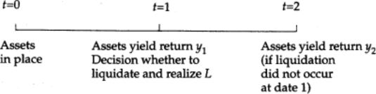
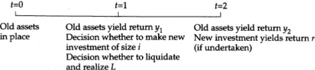
Consider a firm consisting of assets in place, and suppose that it exists at three given dates (see Figure 6.1).
At date 0 the firm's financial structure is chosen. At date 1 the assets in place yield a return of y1. At this time the firm can be liquidated, yielding L (in addition to the y1 already realized). L stands for the value of the firm's assets in some alternative use. The model allows for the possibility that, in some cases, the firm's assets may be more valuable elsewhere.145
If the firm is not liquidated, at date 2 the assets in place yield a
145In the Hart–Moore model of Ch. 5, it was assumed that liquidation was never efficient. However, in the current analysis the manager's private benefit is being excluded from the efficiency calculation. If this private benefit is taken into account, it is never efficient to liquidate in the present model either.
6. CAPITAL STRUCTURE OF A PUBLIC COMPANY |
131 |
Fig. 6.1
further return y2. At this date the firm is wound up, and receipts are allocated to investors.
Note that, in contrast to the last chapter, liquidation is a zero—one decision. A more general treatment would allow for continuous asset sales.
Suppose that the firm is run by a single manager. Recall the assumption that the manager's goal is to maximize the extent of the assets under his control. In model 1 it is assumed that there are no possibilities for the manager to expand his enterprise, and hence the manager's only goal is to avoid liquidation; moreover, once he has achieved this goal, he has no further use for company funds.146
Assume that all uncertainty about y1, y2 and L is resolved at date 1 and there is symmetric information throughout. Assume also a zero interest rate and that investors are risk-neutral.
In a first-best world where contracting is costless, the investors would write the following contract with the manager: CONTRACT 1. Liquidate if and only if y2<L.
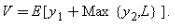
In other words, liquidate if and only if the firm is more valuable (for the investors) liquidated than as a going concern. Such a contract yields the first-best date 0 present value of the firm,147
146This distinguishes model 1 from a ‘pure free cash flow model’ of the Jensen (1986) variety. (A Jensen-type analysis is provided in model 3.) In a pure free cash flow model, the manager always has further uses of company funds and so will squander each dollar of investor returns that is not mortgaged to creditors. Thus, in a free cash flow model the value of equity is zero. In contrast, in model 1, as readers will shortly see, the value of equity can be positive. Note that this is not a critical difference between the two analyses since the main results would still hold under the more extreme Jensen assumptions.
147 Given the simplifying assumption that the manager is interested only in power and not in money (see § 1), wages paid to the manager can be ignored. It is also supposed that the manager has no initial wealth and so cannot be charged up front for non-pecuniary benefits.
132 |
II. UNDERSTANDING FINANCIAL STRUCTURE |
(6.1)
The analysis will focus on a second-best situation where y1, y2, L, although observable, are not verifiable and hence cannot be made part of an enforceable contract. In particular, contract 1 cannot be enforced since the courts do not know whether or not y2<L.148
I consider the role of financial structure in substituting for an enforceable contract. Suppose that, although y1, y2, L are not verifiable, the amount paid out to investors is verifiable. (Any payment made to investors is a public event.) Thus, securities can be issued at date 0 with claims conditional on the amount that is paid out. For the time being, confine attention to the case where the firm issues short-term debt due at date 1, long-term debt due at date 2, and equity; and suppose also that both kinds of debt are senior, in the sense that any new claims issued by the firm at date 1 are entitled to payment only if date 0 debt-holders have been fully paid off. The role of more sophisticated securities is considered below.
As mentioned above, I also assume that, if the firm defaults on its short-term debt at date 1, then this triggers bankruptcy, which in turn leads to liquidation, i.e. L is earned.149
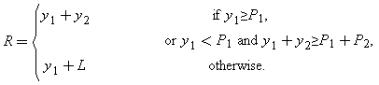
Consider the situation faced by the manager at date 1 once the uncertainty about y1, y2, and L is resolved. Define P1 to be the amount owed at date 1 and P2 to be the amount owed at date 2; i.e., P1 and P2 are the face values of short-term and long-term debt respectively. (Of course, at date 0 these debt claims will typically trade for less than their face value because of the risk of default.) Given that default leads to bankruptcy and to the loss of control benefits, the manager never defaults voluntarily. If y1≥P1, the manager will pay P1 to creditors at date 1 and hold y1−P1 inside the firm for distribution at date 2. Thus the total return to initial shareholders and creditors will be y1+y2, with creditors receiving P1+Min{P2, y1−P1+y2} and shareholders the rest.
Suppose next that y1<P1. If y1+y2≥P1+P2, the manager can still avoid default at date 1 by issuing an amount (P1−y1) of junior debt due at date 2 and repaying this together with the senior debt
148 |
It is one thing to verify L if liquidation occurs at date 1, but it is quite another to verify it in the absence of liquidation. See Ch. 5, n. 8. |
149 |
I ignore more sophisticated bankruptcy systems that try to preserve the firm's going-concern value. Such mechanisms are the subject of Ch. 7. |
6. CAPITAL STRUCTURE OF A PUBLIC COMPANY |
133 |
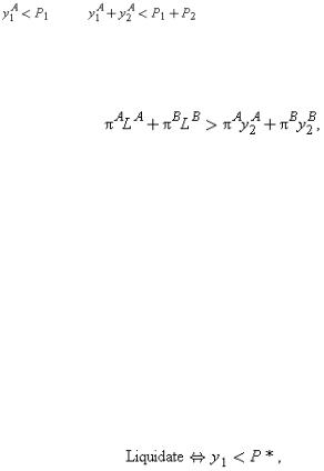
P2 out of date 2 income y2. Thus, the total return to shareholders and creditors is again y1+y2, of which senior creditors receive P1+P2 and shareholders the rest. (Junior creditors put in P1−y1 and get P1−y1 back.) However, if y1<P1 and y1+y2<P1+P2, then the manager cannot avoid default, and liquidation will occur. In this case, the return to creditors is Min{P1+P2, y1+L} and shareholders receive the rest.
Denote the total return to initial shareholders and creditors by R. Then the above discussion can be summarized as follows:(6.2)
Notice for future reference the two sources of inefficiency here. Sometimes the manager will liquidate even though y2>L, because P1 and P2 are large relative to y1 and y2. Other times he will maintain the firm as a going concern even though y2<L, because P1 and P2 are small relative to y1 and y2.
I can now discuss optimal capital structure. Suppose that the firm's capital structure—that is, P1 and P2—is chosen at date 0 to maximize the firm's date 0 market value, that is, the aggregate expected return to all initial security holders: E[R]. This may seem counter-intuitive, given that capital structure decisions are typically made by management (or the board of directors), and I have supposed management to be interested in preserving its empire rather than in market value. The assumption can be justified in two ways. First, the capital structure choice may be made, prior to a public offering at date 0, by an original owner who wishes to maximize his total receipts in the subsequent offering of debt and equity. (He is about to retire.) Second, one can imagine that the firm is all equity prior to date 0, and the threat of a hostile takeover at date 0 forces management to choose a new capital structure which maximizes date 0 market value. (The hostile bidder is present now, but may not be around at date 1, so management must ‘bond’ itself now to act well in the future since otherwise shareholders will sell to the bidder.)150
150Both of these scenarios are of course special. I believe that the thrust of the analysis applies also to the case where management chooses financial structure to maximize its own welfare. In the present three-date model, this leads to the trivial outcome of no debt. (Management clearly prefers not to be under pressure from creditors.) However, in a model with more periods management may issue debt voluntarily, since this may be the only way to raise funds from investors concerned that their claims may be diluted if management undertakes bad actions in the future.It would also be interesting to extend the analysis to show that debt has a bonding role when there is a constant probability of a hostile take-over bid (rather than a probability 1 of a bid now and a probability 0 of a bid at date 1). For a model suggesting that debt does have a bonding role under these conditions, see Zwiebel (1994).
134 |
II. UNDERSTANDING FINANCIAL STRUCTURE |
In the case where there is no ex ante uncertainty about y2 and L, the choice of capital structure is simple. If y2>L, it is optimal to set P1=0.151 If y2<L, it is optimal to set P1 very large. (P2 is irrelevant in both cases.) The return to shareholders is V0=max{y1+y2, y1+L} and so the first-best is achieved.
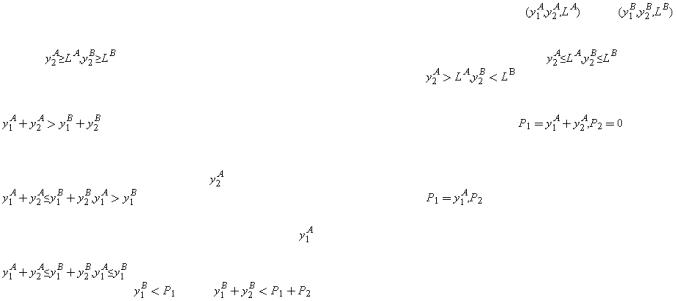
Matters become more interesting if y2 and L are uncertain. (Whether y1 is uncertain or not is less important.) To simplify, focus on the special case in which the vector (y1, y2, L) can take on just two values, and , with probabilities πA and πB=1−πA, respectively.
Obviously, if |
, the first-best outcome can again be achieved with no date 1 debt; if |
, the first- |
||||
best can be achieved with a high level of date 1 debt. The interesting case is |
(or vice versa). It is useful |
|||||
to divide this case into three subcases. |
|
|
|
|
||
1. |
. Here the first-best can again be achieved, for example by setting |
. That is, |
||||
short-term debt is set equal to the total value of the firm in state A. The reason is that in subcase 1 the state in |
||||||
which total return is low is also the state in which the firm should be closed down. Hence the firm can avoid |
||||||
default in state A (by borrowing |
) but not in state B. This is the efficient outcome. |
|
||||
2. |
|
. Now the first-best can be achieved by setting |
very large. The reason is that in |
|||
subcase 2 the state in which date 1 return is low is also the state in which the firm should be closed down. Hence |
||||||
the firm can avoid default in state A (by paying |
) but not in state B (since it can't borrow any more). Again, |
|||||
this is efficient. |
|
. Now the first-best cannot be achieved. Given any values of P1, P2, default in state B |
||||
3. |
|
|||||
occurs if and only if |
and |
|
(see (6.2)). But these |
|
|
|
151 Recall the assumption that the manager has no use for company funds if liquidation is avoided. Hence, conditional on the fact that liquidation is undesirable, there is no cost to setting P1 very low (zero).
|
6. CAPITAL STRUCTURE OF A PUBLIC COMPANY |
135 |
|
inequalities imply that |
and |
, and hence default also occurs in state A. It is impossible to |
|
have liquidation in state B, where liquidation is efficient, without also having it in state A, where it is inefficient. Thus, the choice is between having liquidation in both states or neither. The first, which can be achieved by setting P1 very large, is preferable to the second, which can be achieved by setting P1=0, if and only if(6.3)
i.e. if and only if the expected liquidation value exceeds the expected continuation value.
This completes the analysis of optimal capital structure in the two-state case. The main difference relative to the case of perfect certainty is that interior solutions occur: it may be optimal to choose debt levels to take intermediate values (subcases 1 and 2) rather than zero or infinity. Also, high debt sometimes leads to inefficient liquidation and low debt sometimes prevents efficient liquidation (see subcase 3).152
It is worth considering how financial structure differs from an incentive scheme as a way of controlling management. As noted earlier, since y1, y2, L are not verifiable, state-contingent incentive schemes are not feasible. Also, an incentive scheme that rewards the manager for liquidating will not be effective given the assumption that the manager puts power before money. However, the following incentive scheme could be useful: the firm's capital structure consists of equity and no debt, the manager is not allowed to raise new capital, and the manager is dismissed at date 1 unless he pays a dividend to shareholders of at least P*.
Note, however, that such a scheme yields a liquidation rule
which is equivalent to that obtained by choosing debt levels
152At this stage, it is worth reviewing the assumption that renegotiation with creditors is impossible. If one were to take the opposite point of view—that renegotiation is
costless, as in Ch. 5 —one would find that P1 =∞ is optimal (assuming that one retained the assumption that capital structure is chosen to maximize investor return). The reason is that, with P1 =∞, investors have the right to insist on liquidation in those states where liquidation is efficient; and at the same time, they can always renegotiate P1 downwards in those states where liquidation is inefficient. Thus, the assumption that renegotiation is costly plays a very important role in model 1.

136 |
II. UNDERSTANDING FINANCIAL STRUCTURE |
P1=P*, P2=∞. In general, however, one can do better with a more flexible capital structure—in particular, by setting P2<∞ (see subcase 1). The reason is that when P2<∞ the liquidation rule
depends on y2 as well as y1. That is, debt, coupled with the manager's ability to refinance at date 1, yields an outcome that is sensitive to y2 in a way that is not possible with the simple incentive scheme considered above.153
3.Model 2
Model 1 is concerned with a situation where the only issue is whether the firm should shrink. Under these conditions, short-term debt is of primary importance (to trigger liquidation), while long-term debt is somewhat less important. Model 2 allows for the possibility of expansion. This provides a more interesting role for long-term debt as a means of regulating the inflow of new capital.154 Unfortunately, it is difficult to combine liquidation and new investment, and so model 2 makes a simplifying assumption (see Assumption 1 below). This assumption implies that it is optimal to set short-term debt equal to zero, so that no liquidation occurs in equilibrium. The analysis can therefore focus on longterm debt.
The timing is as before, except that at date 1 the firm may undertake an investment project (see Figure 6.2). The project costs i and yields r at date 2. The variables i and r are uncertain as of date 0, but the uncertainty is resolved at date 1.
The manager's empire-building tendencies are such that he always wants to invest if he can. That is, just as the manager wants to avoid liquidation at all cost, so he wants to invest at all cost. The only thing that can stop him is an inability to raise the capital. However, as in model 1, once the investment is financed, the manager has no further use for company funds.
It is assumed that claims cannot be issued on the return from
153I have not allowed investors to send messages about the commonly observed values of y1 , y2 , and L. Messages would be an alternative way of making the liquidation rule sensitive to y2 . See e.g. Moore (1992).
154Model 2 is based on Hart and Moore (1995).
6. CAPITAL STRUCTURE OF A PUBLIC COMPANY |
137 |
Fig. 6.2
the investment, r, separately from the return from the assets in place, y2; that is, project financing is ruled out.155 I also make an assumption that implies that it is optimal to set P1=0, so that no liquidation occurs in equilibrium.
ASSUMPTION1. y1<i and y2≥L with probability 1.
Assumption 1 says that the manager can never finance the investment out of date 1 earnings and that it is never efficient to liquidate the firm. The assumption may be plausible for a growth company that, at least initially, requires an injection of new capital to prosper.
PROPOSITION 1. Given Assumption 1, the date 0 market value of the firm is maximized by setting P1=0.
The following is a sketch of the proof (for details, see Hart and Moore 1995). Given any choice of (P1+P2), it is better to replace P1 by zero and P2 by (P1+P2). The reason is that a zero value of P1 makes liquidation (which is inefficient) less likely. Also, a zero value of P1 does not make it easier for the manager to invest in a bad project, since, given that y1<i, the manager has to go to the market, in which case only the total amount of senior debt in
155 If project financing were possible, the new investment could be financed as a stand-alone entity, whose merit could be assessed by the market at date 1; and debt levels could be set very high to prevent the manager using funds from the existing assets to subsidize investment. There are several justifications for ruling out project financing. First, it may be that i represents an incremental investment—e.g. maintaining or improving the existing assets—and the final return y2 +r is simply the overall return from the (single) project. Second, it may be that the same management team looks after both the old assets and the new project, and can use transfer pricing to reallocate profits between them; hence the market can keep track only of total profits. Finally, even if project-specific financing is feasible, it is not at all clear that management will want to finance a project that is not part of its empire since it will not enjoy the private benefits of control (on this, see Li 1993).
138 |
II. UNDERSTANDING FINANCIAL STRUCTURE |
place—P1+P2—is important for determining the amount of capital he can raise. (See the argument leading to (6.4) below.) This establishes the proposition.
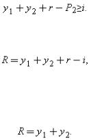
Given that P1=0, and no liquidation occurs, the analysis of model 2 is relatively simple. The firm's total revenue if the manager invests is y1+y2+r, of which P2 is mortgaged to the old (senior) creditors. Hence, the most the firm can borrow at date 1 is y1+y2+r−P2. It follows that the manager will invest if and only if(6.4)
If (6.4) is satisfied, the total return to date 0 investors, R, is(6.5)
of which date 0 creditors receive P2 and shareholders receive the rest. (New creditors are paid back in full.) If (6.4) is not satisfied, the total return to date 0 investors is(6.6)
Notice the two sources of inefficiency in model 2. Sometimes the manager will invest even though r<i, because y1+y2 is big relative to P2. At other times he will be unable to invest even though r>i, because y1+y2 is small relative to P2. (The latter is known as the debt overhang problem; see Myers (1977).)
It is now straightforward to analyse optimal capital structure in model 2. If there is no ex ante uncertainty about i and r, it is easy to achieve the first-best outcome. If r>i, set P2=0; (6.4) is always satisfied and investment takes place, which is efficient. In contrast, if r<i, set P2 very large; (6.4) is never satisfied and investment never takes place, which is again efficient.
Matters become more interesting if r and i are uncertain. To simplify, again suppose that (y1, y2, r, i) takes on just two values,  and
and  , with probabilities πA and πB=1−πA, respectively.156
It is again trivial to achieve the first-best outcome with no debt if rA≥iA and rB≥iB, or with very large debt if rA≤iA and rB≤iB. The interesting case is where rA>iA and rB<iB. Divide this into two subcases.
156 For an analysis of the case with more than two states, see Hart and Moore (1995).
|
6. CAPITAL STRUCTURE OF A PUBLIC COMPANY |
139 |
1. |
. That is, the firm's net market value and the profitability of the new project |
|
are perfectly (positively) correlated. Here the first-best can be achieved by setting P2 |
somewhere between |
|
and |
; (6.4) is satisfied in state A but not in state B, and investment occurs only |
|
in state A, which is efficient.
In other words, setting the debt level somewhere between the maximized net value of the firm in state A and the
|
maximized net value in state B gives management enough leeway to finance a profitable new investment in state |
2. |
A, but prevents the financing of an unprofitable one in state B. |
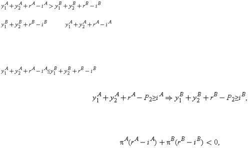
. That is, the firm's net market value and the profitability of the new project are |
|
|
perfectly (negatively) correlated. The first-best is no longer achievable for any choice of P2. The reason is that |
and so it is impossible to have investment in state A without also having it in state B. Thus, the choice is between having investment in neither state (set P2 very large) or in both (set P2=0). The first is preferable if and only if
i.e. if and only if the expected net return from new investment is negative.
The lesson from this second model complements that from the first. If management is interested in empire-building, the danger for investors is that management will try to raise capital for unprofitable investment projects by issuing claims against earnings from existing assets. Senior long-term debt, by mortgaging part of long-term earnings, reduces management's ability to do this. However, too much long-term debt prevents managers from carrying out even those projects that are profitable.
This chapter has restricted attention to ‘simple’ capital structures consisting of fixed amounts of senior debt. It is not difficult to show, however, that in some cases more sophisticated securities can be useful. Consider model 2 and suppose that y1≡0 and y2≡r. (That is, the return from assets in place and the return from new investment are always the same.) Then the first-best can be achieved in the following way. The firm issues a large class of senior debt due at date 2 in the amount of K, say, with a covenant