

Учебный год 22-23 / Firms, Contracts, and Financial Structure
.pdf110 |
II. UNDERSTANDING FINANCIAL STRUCTURE |
implying that the amount left of L1 (the initial loan) which can be used to buy project assets—the debt capacity—is
In other words, E must finance the difference, K−M, out of his initial wealth w. But this is precisely what (5.16) tells us.
As noted, there is a continuum of feasible repayment paths. Once (a reasonable amount of) uncertainty is introduced, the multiplicity will typically disappear (see § 4). Another way to break the multiplicity is to suppose that E and C have reinvestment opportunities over and above those represented by the project. For example, suppose E can reinvest any extra money he has (including cash flows from the project) at a positive interest rate, whereas reinvestment by C occurs at the market interest rate of zero. Then it is not difficult to show that the unique optimal repayment path is the slowest one. The reason is that this gives E the maximum ability to make additional reinvestments, which contribute to total surplus. On the other hand, if C can reinvest at a positive interest rate, whereas E faces a zero interest rate, then the unique optimal repayment path is the fastest one, since this gives C the maximum ability to make additional reinvestments. (For details, see Hart and Moore (1994a).)
In the case of no reinvestments, (5.16)–(5.18) can be used to obtain further insight into the kinds of project that will be financed, and the determinants of the repayment paths.
DEFINITION 1. The assets become longer lived, or more durable, if Lt increases for all 1≤t≤T−1. DEFINITION 2. The project returns become more front-loaded if  increases for all 1≤t≤T.
Note that the second definition is consistent with |
staying the same; that is, although the returns arrive more |
quickly, the total value of the project may be constant. |
|

5. FINANCIAL CONTRACTING AND DEBT |
111 |
It is now easy to use (5.16)–(5.18) to establish the following:
AIf the project assets become more durable, then the project is more likely to be undertaken (the right-hand side of (5.15) increases for all t and so the right-hand side of (5.16) decreases) and the slowest repayment path
becomes slower |
increases for all t=1, . . . ,T). |
BIf the project returns become more front-loaded, then the project is more likely to be undertaken (the left-hand side of (5.15) decreases for all t and so the right-hand side of (5.16) decreases) and the fastest repayment path become faster  decreases for all t=1, . . . ,T).
As a conclusion to this section, it is useful to consider some of the empirical evidence about the determinants of debt contracts and maturity structure.122 The evidence suggests that long-term loans are used for property, leasehold improvements, machinery, and the like. Also, debt with the longest term is typically on property: real estate mortgages. Short-term loans, on the other hand, tend to be used for working capital purposes—e.g. payroll needs, the financing of inventory, and the smoothing of seasonal imbalances. Moreover, the collateral is usually made up of assets such as the inventories or the accounts receivable.123
The analysis is consistent with the evidence. The analysis has shown that, if assets are long-lived, they will support long-term debt. Property and machinery are obvious examples of highly durable assets. Conversely, if the assets are short-lived, as in the case of inventories (which may not retain their value, or which can be disposed of relatively easily) or accounts receivable, then the debt is likely to be short-term.
The evidence on short-term financing is also consistent with result B, i.e. that the faster the returns arrive, the shorter will be the maturity of debt (in the fastest path). A firm that is raising money for payroll needs, for purchasing inventory, or for smoothing seasonal imbalances, is typically the kind of firm whose returns will be coming in soon.
There is also evidence suggesting that the amount of ‘equity’ an entrepreneur has to put into the project himself, and the value of
122For a more detailed exposition of what follows, see Hart and Moore (1994a).
123See Dunkelberg and Scott (1985: tables 6, 7, 10, 12, and 13) and Dennis et al. (1988: table 3.11).
112 |
II. UNDERSTANDING FINANCIAL STRUCTURE |
the collateralized assets, are important factors in determining whether a project is financed.124 This finding is hardly surprising, but it fits in well with the model, in light of result (A) and the fact that w is a crucial variable in determining whether (5.16) is satisfied.
Finally, the model can explain the conventional wisdom among practitioners that ‘assets should be matched with liabilities’. To be precise, it has been shown that liabilities (namely the debt repayments P1, P2, . . . ,PT) should be matched either with the return stream (y1, y2, . . . ,yT) (in the case of the fastest repayment path), or with the rate of depreciation (l1, l2, . . . ,lT−1) (in the case of the slowest repayment path).125
I am not suggesting that the above evidence is hard to explain or that other theories cannot explain it. However, it is perhaps a selling point of the model that, as well as being simple and tractable, it can be used to understand the basic facts about maturity structure.
4.The Case of Uncertainty
Sections 2 and 3 showed that in the case of perfect certainty (without reinvestment opportunities) there is a continuum of feasible repayment paths, and an even larger class of optimal debt contracts. One way to reduce or eliminate the indeterminacy is to introduce uncertainty. Unfortunately, the uncertainty case is not yet very well understood, and so I will provide only a brief discussion. (This section is based on Hart and Moore (1989).)
124 See the regularly featured articles ‘Lending to . . . ’ in the Journal of Commercial Bank Lending. Also see Dunkelberg and Scott (1985: tables 1, 2, 12, 13), Dennis et al. (1988: table 3.7). and Smollen et al. (1977: 21). For more formal empirical work on the determinants of debt levels, see Long and Malitz (1985) and Titman and Wessels (1988).
125There is an important caveat. The analysis has concentrated on equilibrium repayment paths. As noted, in a deterministic model one can, without loss of generality, focus on debt contracts that are never renegotiated. However, other contracts, which are renegotiated, could have yielded the same intertemporal allocation, e.g. a contract consisting of a large amount of short-term debt that is rolled over. Thus, in terms of the empirical evidence, the analysis has actually explained the maturity of repayment paths rather than the maturity of the debt contracts themselves.
5. FINANCIAL CONTRACTING AND DEBT |
113 |
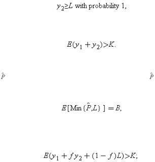
Return to the two-period model (Section 2). Suppose now that the variables y1, y2, L are uncertain at date 0, but that their realizations are learned by both parties at date 1. (There is symmetric information throughout.) However, although y1, y2, and L are observable, they are not verifiable, and so state-contingent debt contracts cannot be written. In addition, both parties are risk-neutral. Make the following generalizations of (5.2)–(5.3):(5.20)
(5.21)
(Here E denotes the expectations operator.)
Denote a debt contract by (B, ), where B≥K−w is the amount borrowed and is the amount owed at date 1. Since all uncertainty is resolved at date 1, equations (5.4) and (5.6) still apply. The condition for C to break even is now(5.22)
where the expectation is taken with respect to L. The condition for E to participate is E [B−(K−w)+y1−Min(B−(K−- w)+y1, P)+fy2]>w, where  . Given (5.16) and (5.22), this can be simplified to(5.23)
i.e., the project has positive expected net present value, when account is taken of the fact that some liquidation occurs at date 1. Another way to understand (5.23) is to note that E's payoff (net of his initial wealth w) plus C's net payoff equals the expected net present value of the project; since C breaks even, it follows that E's (net) payoff is
E[y1+fy2+(1−f)L]−K.
I now present two examples. In the first it is optimal to set B=K−w. In the second it is optimal to set B>K−w. The examples stand in contrast to the case of certainty where B=K−w and B>K−w are typically both optimal (if L>K−w).
Example 3. |
Suppose K=90, w=50 and there are two equally likely states: |
|
|||
|
State 1: |
|
y1=50, |
y2=100, |
L=80. |
|
State 2: |
|
y1=40, |
y2=100, |
L=30. |
Consider the contract B=K−w=40 and P=50. In state 1, E repays 50. In state 2, E renegotiates the payment down to 30. C's average
114 |
II. UNDERSTANDING FINANCIAL STRUCTURE |
return is 40, and hence C breaks even. In both states f =1, i.e. the first-best is achieved and there is no inefficiency.
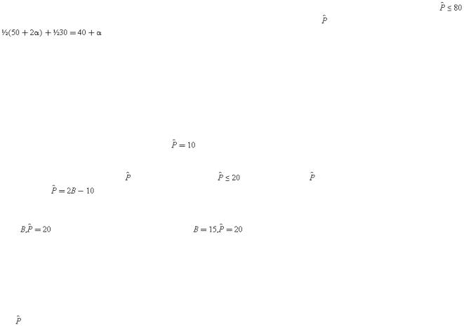
Now consider a contract where B=40+α, and α>0. Then C will be fully repaid in state 1 (as long as |
), but will |
|
receive only 30 in state 2. Hence, in order for C to break even, |
must equal 50+2α. (C |
then receives |
.) But E's wealth in state 1 is only 50+α (50 from the project return plus α held over from date 0). Thus, there will be liquidation in state 1 and the first-best is not achieved.
The next example shows that B>K−w may be optimal.
Example 4. |
Suppose K=20, w=10, and there are two equally likely states: |
||||||||
|
State 1: |
|
y1=0, |
|
|
y2=20, |
|
L=20. |
|
|
State 2: |
|
y1=0, |
|
|
y2=40, |
|
L=10. |
|
Consider the contract B=K−w=10 and |
. C receives 10 in both states from liquidation sales. (E has no cash.) In |
||||||||
state 1, f =0.5. In state 2, f =0. E's expected return=E(fy2)=0.5(0.5)20=5. |
|
|
|
||||||
Now consider a contract (B, ), where B>10 and |
. C will receive |
in state 1 and 10 in state 2, and so for C to |
|||||||
break even |
. In state 1 E pays over B−10 (his remaining wealth) and f =1−B/20 (so B is generated in asset |
||||||||
sales). In state 2 E pays over B−10 and f =(B−10)/10 (so 20−B is generated in asset sales). C breaks even and E's
expected return=E(fy2)=(1/2)(1−B/20)20+(1/2)[(B−10)/10]40=3B/2−10, which achieves a maximum at B=15. (At |
||
this |
.) Thus, the optimal contract is |
. E's expected return=12.5. |
Basically, what's going on here is that it helps when E has some wealth left over from date 0 since this allows him to ‘buy back’ the assets at date 1, with a considerable reduction in inefficiency in state 2. (Liquidation does not matter in state 1 since, given that y2=L, it has no social cost.)
In future work, it would be desirable to obtain some general results about the nature of the optimal debt contract for the case of uncertainty. One difficulty is that it is not clear that attention should be confined to contracts of the form (B, ). For example, it might be optimal to arrange that in default states E should receive some part of the liquidation receipts, in order to encourage E and
5. FINANCIAL CONTRACTING AND DEBT |
115 |
C to renegotiate in a ‘more efficient manner’.126 Another idea is to make E the owner of the project, but give C an option to buy E out at a specified price.127 Figuring out the class of feasible contracts when there is uncertainty is an important, but difficult, topic for future research.
5.Multiple Investors and Hard Budget Constraints
The analysis has so far considered the case of one investor. In reality, of course, there will often be more than one. This might be because no investor is rich enough to finance the project alone, or because no investor wishes to bear the risk of financing the project alone (if investors are risk-averse). There is another reason for multiple investors, however: to harden E's budget constraint.128
To understand this idea, return to the two-period model of Sections 2 and 4. In the one-investor case the entrepreneur may default even when he can pay his debts, in order to renegotiate the debt payment down to L. Unfortunately, such a strategic default can have undesirable ex ante consequences. In particular, it puts a ceiling on the investor's return from the project and may deter the investor from financing certain projects.129
It has been pointed out in the literature that multiple investors may make strategic default less attractive (see e.g. Bolton and Scharfstein 1994).130 The basic idea is that renegotiation is more likely to break down with multiple investors—because of
126This idea is explored by Harris and Raviv (1995).
127For example, suppose K =300, w =260, and there are three states. In state 1 (probability 1/10), y1 =10, y2 =200, L=105. In state 2 (probability 2/5), y1 =10, y2 =20, L =80. In state 3 (probability 1/2), y1 =50, y2 =200, L =200. Then a (B, P ) contract does not achieve the first-best. However, the following ‘option-to-own’ contract does: E puts 260 into the project and is the owner in all states of the world. However, C has the option to buy the project assets for 120. With such a contract, C will exercise her option only in state 3, where there are no social costs of liquidation. In addition, C breaks even under the contract.
128The notion of a hard budget constraint is due to Kornai (1980).
129For instance, take example 2 but suppose that y2 =70. Then in the absence of renegotiation a debt contract with repayment P =60 achieves the first-best: E can afford the repayment and prefers to pay rather than face liquidation, and C breaks even. In contrast, in the presence of renegotiation, E will default and beat C down to 30. Anticipating this, C refuses to finance the project.
130A related idea is explored in Dewatripont and Maskin (1990).
116 |
II. UNDERSTANDING FINANCIAL STRUCTURE |
free-rider and hold-out problems combined with asymmetric information—and so the entrepreneur may simply choose to pay P even when P>L.
A simple way to understand this is to consider the case where there are N investors, each owed P/N. Suppose E defaults and makes the following (take-it-or-leave-it) offer to the investors: ‘I propose that at least M of you agree to forgive your debt down to (slightly above) L/N. Otherwise bankruptcy and liquidation will ensue.’ Then each investor should reason as follows: ‘My decision to forgive my debt is very unlikely to be pivotal in determining whether the critical number M agrees to forgive. (With a small amount of noise, the probability that any investor is pivotal can be shown to tend to zero as N→∞ if M/N is bounded away from zero and from one.) If I think that at least M investors will forgive, I am better off not forgiving since E will then have to pay me the full amount P/N. If I think the critical number M will not forgive, then there is certainly no advantage to my forgiving and there may be a disadvantage if I have a claim in bankruptcy to L/N rather than P/N.’
Given this logic, no creditor will accept E's offer, and E's attempt to reduce the debt will fail. Moreover, anticipating this, E will pay the full amount owed, P.131
Unfortunately, the inflexibility exhibited by a large number of creditors deters not only strategic default, but also productive renegotiation. Consider example 3. In state 2, E cannot pay his debt of 50. In the absence of renegotiation, liquidation would occur at a social cost of y2−L=70. With renegotiation, the debt is reduced to 30 and a more efficient outcome is achieved. However, it may be difficult to persuade a large number of creditors to reduce the debt from 50 to 30. The reason is similar to that given above. Each creditor will argue that her decision to forgive is unlikely to be pivotal in determining whether the renegotiation succeeds. If the creditor expects enough other people to forgive, it
131 For formalizations of this idea, see Aggarwal (1994), Gertner and Scharfstein (1991), Holmstrom and Nalebuff (1992), Mailath and Postlewaite (1990), and Rob (1989). One strategy the entrepreneur might adopt is to require unanimous acceptance of his offer, i.e. to set M =N, thus making each creditor pivotal. However, when there are many creditors unanimity is hard to achieve: it takes only one (‘crazy’) creditor with a different belief from the others (e.g. the creditor might think the liquidation value of the project is substantially above L ), or a different agenda, to defeat a unanimity offer.
5. FINANCIAL CONTRACTING AND DEBT |
117 |
is better for her not to forgive (i.e. to hold-out or free-ride) since that way she gets her full 50/N. On the other hand, there is certainly no reason to forgive in the event that the renegotiation fails. Since each creditor thinks the same way, a socially desirable renegotiation fails.132
So there are costs and benefits from having multiple investors. Multiple investors are good at deterring strategic default but bad at preventing productive renegotiation.133 It may be possible to develop a theory of the optimal number of creditors along these lines.134
So far I have considered the case of multiple investors with the same claim. Another interesting line of research—due to Dewatripont and Tirole (1994) and Berglöf and von Thadden (1994)—looks at multiple investors with different types of claims. This is discussed briefly below.
132 It is not being suggested that debt renegotiations always fail in practice. However, Gilson et al. (1990), in a study of the companies listed on the New York and American Stock Exchanges that were in severe financial distress during 1978–87, found that workouts fail more than 50 per cent of the time and are more likely to fail the larger the number of creditors. See also Gilson (1991) and Asquith et al. (1994), and, for a survey of financial distress, John (1993). One way to make debt renegotiation easier is to include a provision in the initial debt contract that the aggregate debt level can be reduced as long as a majority of creditors approve (i.e. the majority's views are binding on the minority). (It turns out that the Trust Indenture Act of 1939 makes such a provision illegal in the USA for public debt.) The problem with such an arrangement is that, when there are large numbers of creditors, no individual creditor has a strong incentive to vote ‘intelligently’ (i.e. to incur the cost of collecting information about the firm's financial position), or even to vote at all, since her vote is unlikely to affect the outcome. Thus, one cannot be confident that creditors will be able to distinguish between situations of involuntary default, where debt forgiveness should be encouraged, and situations of strategic default, where it should be resisted.
133In arguing that multiple creditors will deter strategic default, I have supposed that E loses control of the project if it is liquidated. However, it is not uncommon for a delinquent debtor to buy back project assets in a liquidation sale (for something close to L ). If this strategy is open to E, then he faces a soft budget constraint however many creditors there are.
134Leveraged buy-out transactions may be cases where the benefits of a hard budget constraint are large relative to the costs. In these transactions a company is purchased, often by incumbent management, through the issuance of debt to a large number of investors. A desirable feature of such transactions is that managers have a strong incentive to work hard since, if they do not, they risk bankruptcy. Leveraged buy-out transactions were particularly popular in the USA in the 1980s (see Jensen 1989).
118 |
II. UNDERSTANDING FINANCIAL STRUCTURE |
6.Related Work
There is a considerable literature on financial contracting that is related directly or indirectly to the work described above. Unfortunately, I have space to mention only a few contributions and themes. The Bolton—Scharfstein (1990) paper has already been noted. This paper develops a model that is similar in many ways to the Hart—Moore (1989) model; the main difference is that the penalty for nonpayment of debt is that the creditor withholds future finance rather than liquidating existing assets.135 I have also mentioned the costly state verification model of Townsend and Gale-Hellwig—a detailed analysis of which is provided in the Appendix. The CSV model is based on comprehensive contracting ideas but it shares the feature of both the Hart—Moore and Bolton—Scharfstein models that a debtor pays his debts only because he will be penalized otherwise. In the CSV model, however, the penalty is that the debtor is inspected.
Although most of the analysis of this chapter has been concerned with debt levels rather than with debt maturity, the structure of repayment paths for the special case where returns and liquidation values are perfectly certain was also studied. A rather different approach to debt maturity is contained in some interesting work by Diamond (1991). Diamond analyses the trade-off between short-term and long-term debt in a two-period model which combines asymmetric information and incomplete contracts. He argues that an entrepreneur who knows that his project is profitable will finance it with short-term debt—with the intention of refinancing later on when new information arrives—while an entrepreneur who knows that his project is unprofitable will use long-term debt. The reason is that the ‘high-quality’ entrepreneur is prepared to bear the risk that the new information about the project's profitability will be adverse, and that the project will therefore not be refinanced, while the low-quality entrepreneur is not prepared to bear this risk.136
135 |
Neher (1994) explores the idea that creditors can threaten to withhold future finance in a dynamic model of a start-up venture. |
136 |
The idea that an agent may use the contract he writes to signal something about his type may also be found in Aghion and Bolton (1987) and Hermalin (1988). |
5. FINANCIAL CONTRACTING AND DEBT |
119 |
One benefit of the Diamond approach is that it pins down the optimal contract as well as the optimal repayment path. (In contrast in the perfect certainty model analysed in Section 3, there were many optimal contracts, most of which were renegotiated along the equilibrium path.) However, it is not clear how easy it is to generalize the model to many periods.
The chapter briefly considered the role of multiple investors in hardening the entrepreneur's budget constraint. The analysis focused on the case of identical creditors. Another possibility is to have investors with different claims. Two interesting papers that explore this theme are Dewatripont and Tirole (1994) and Berglöf and von Thadden (1994). Dewatripont and Tirole consider a model in which the firm's profit is verifiable but the entrepreneur has an unverifiable effort choice. They show that it is optimal to have two outside investors holding debt and equity in different proportions. (Debt-holders and equity-holders are distinguished partly by the fact that they have different claims on verifiable profit.) The basic idea is that, if both investors hold debt and equity in the same proportions, the investors will be too soft on the entrepreneur, i.e. they won't intervene enough. In particular, they won't liquidate the firm if first-period profits are low because the value of continuation may exceed the value of liquidation (as shareholders, they see the upside gains as well as the downside losses). In contrast, if one of the investors holds debt and the firm defaults in the first period, this investor—to whom control now shifts—will be eager to liquidate (since she doesn't see the upside gains from continuation). As a result, the entrepreneur will be forced to make concessions and will also have a strong incentive to avoid default.
Berglöf and von Thadden, in independent but related research, show that similar considerations explain why a firm's short-term and long-term debt should be allocated to different investors. In their analysis, the short-term creditor plays the role of the aggressive creditor in the Dewatripont–Tirole model, while the long-term creditor plays the role of the passive shareholder.
I close this chapter by mentioning two directions for future research. First, the models discussed in this chapter portray equity in a rather rudimentary manner. Either a firm's profit is unverifiable—in which case an equity-holder receives a return only because of her ability to hold up the entrepreneur. (For