Учебный год 22-23 / Firms, Contracts, and Financial Structure

Stochastic control is hard to interpret, but a slight embellishment of the model leads to something more natural.107 Suppose that income from the project, y, depends on a verifiable state of the world θ which is realized after the contract is signed but before a is chosen.108 (The private benefit b is independent of θ.) Assume further that

where α>0,α′<0, z>0. Then it is not difficult to show that the optimal contract has the following form. There is a cutoff θ* such that E has control when θ>θ*. The cut-off is chosen so that C breaks even on average. The intuition behind the cut-off is that, given α′<0, high θ states are those where the choice of action has relatively little effect on y (and so E should control action) and the low θ states are those where the choice of action has a relatively large effect on y (and so C should control action). Note that, if α′(θ)z(a)+β′(θ)>0 for all a A, high θ states are high-profit states, i.e. E receives control when profits are high. However, the opposite is true if α′(θ)z(a)+β′(θ)≤0 for all a A. Then E receives control when profits are low.109

107Stochastic control is not always optimal. The analysis has focused on contracts that allocate all the monetary returns to C. There are other possibilities, however, if (5.1)

holds strictly. For example, C could retain control but give E a lump-sum transfer by way of compensation, equal to y (ac )−K ; E could then use this transfer to bribe C to choose a more efficiently. The advantage of such an agreement is that the action a is deterministic rather than random, which increases total surplus if b or y is strictly

concave. One case where stochastic control can be shown to be optimal (although not uniquely optimal) is if b (a )=λa, y (a )=Y −a, 0≤a ≤a , and λ>1. (Here b and y are not strictly concave and so randomization of action does not reduce surplus.) See also n. 7.

108 This is the case Aghion and Bolton (1992) consider. See also Berglöf (1994).

109Stochastic control is not always optimal. The analysis has focused on contracts that allocate all the monetary returns to C. There are other possibilities, however, if (5.1)

holds strictly. For example, C could retain control but give E a lump-sum transfer by way of compensation, equal to y (ac )−K ; E could then use this transfer to bribe C to choose a more efficiently. The advantage of such an agreement is that the action a is deterministic rather than random, which increases total surplus if b or y is strictly

concave. One case where stochastic control can be shown to be optimal (although not uniquely optimal) is if b (a )=λa, y (a )=Y −a, 0≤a ≤a , and λ>1. (Here b and y are not strictly concave and so randomization of action does not reduce surplus.) See also n. 7.

E can divert or ‘steal’ y1, i.e. that y1 is a potential private benefit. However, E may be persuaded not to divert y1, as will be seen shortly.

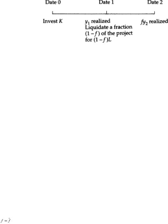
Identify the action a with the choice about whether to continue the project past date 1. More precisely, suppose that a decision must be made about what fraction of the project assets, (1−f), to liquidate (see Figure 5.1). Liquidation of a fraction (1−f) of the project yields a verifiable income (1−f)L at date 1 and a non-verifiable income fy2 at date 2.110 Suppose that E can divert fy2 also, and so the continuation value of the project is another potential private benefit.

Fig. 5.1

The assumption that E can divert y1 and fy2 is of course extreme. It is meant to capture the idea that E has discretion over cash flows, e.g. that he can use them for perks rather than pay them out. With reference to the Aghion–Bolton model, (1−f)L corresponds to the verifiable income y(a) and fy2 to the private benefit b(a).

Suppose that the project terminates at date 2 (the assets are

110 Partial liquidation is permitted for reasons of analytical convenience. If liquidation is a 0 or 1 decision, then the model exhibits discontinuities that are both mathematically and economically troublesome. Note that, although partial liquidation is allowed ex post, the project is supposed to be indivisible ex ante. The analysis could easily be extended to the case of continuous project size, however. Note also that it is assumed that the fraction of the project to be liquidated, (1−f ), is not ex ante contractible. One justification for this is that, if the assets are not truly homogeneous, it may not be clear what liquidating ‘10 per cent’ of the assets means. Thus, a contract that specifies may not be enforceable because it is not precise. Another possibility is to specify that enough assets should be liquidated to realize a specified monetary amount. However, it may be unclear whether the asset sales will yield the specified monetary amount until the assets have been sold (by which time it is too late to do anything about

it if the monetary amount has not been realized).

worthless then), and the interest rate is zero. Allow also now for the possibility that the entrepreneur has some initial wealth w, where w<K (w could be zero).

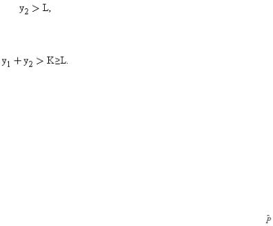
The analysis of this and the next section will be concerned with the case where y1, y2, and L are perfectly certain. Assume(5.2)

(5.3)

Inequality (5.2) says that it is always first-best efficient not to liquidate the project. (So, in the Aghion–Bolton terminology, the first-best optimal action a*=f*=1.) Inequality (5.3) says that the project has positive net present value, and that the assets depreciate.

The first point to note is that there is no way to get E to pay out any of the date 2 receipts, fy2, to C. The reason is that whatever part of fy2 E has promised to C, E will default, diverting fy2 to his own account. C has no leverage over E at date 2 since the project is over and the assets are worthless.111

In contrast, it is possible to get E to pay over part of y1 to C. At this stage the project is still worth something to E. If the consequence of not making a payment is the loss of control of the project, then E may prefer to make the payment.

This suggests consideration of the following debt contract. E borrows B≥K−w at date 0 and promises to repay at date 1. If E makes the repayment, he keeps control and has the right to continue the project until date 2. If E doesn't make the repayment, C has the right to terminate the project, in which case it is supposed that she receives all the liquidation receipts.112 However, C may choose not to exercise her liquidation right; that is, renegotiation may take place.113 As in the Aghion–Bolton model, it will be

111I rule out the possibility that C can get E convicted of theft if E does not repay fy2 . One justification is that there may be a small amount of uncertainty in the background, so that E can always claim that y2 =0.

112More complicated contracts could be conceived in which the liquidation receipts are divided in some pre-specified manner. Allowing these would not affect the analysis in the case of perfect certainty.

113It is assumed that the investor cannot run the business by herself and thereby realize the returns y1 , y2 . I take the point of view that the investor would have to hire a substitute manager, who could also divert y1 and y2 . The best the investor can do by herself is to liquidate the assets for L.

supposed that E has all the bargaining power in any ex post renegotiation, as well as at date 0.

Analysis of the Optimal Debt Contract

Make the simplifying assumption that E can liquidate assets himself at date 1 (without C's permission) in order to meet the debt payment .114

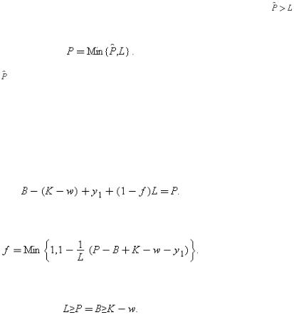
Since E has all the bargaining power, C will never receive more than L at date 1.115 In particular, if , E will default at date 1 and beat C down to L in the renegotiation. That is, whatever is chosen in the contract, C will receive(5.4)

Since only P is relevant, rather than , in what follows I represent a debt contract by the two numbers B and P (here P is the actual repayment), where P≤L.

The next question to ask is: in what form is P received? Given (5.2), E has an incentive to pay as much as possible of P in the form of cash and as little as possible in the form of asset sales, i.e. liquidation. E's date 1 cash holding equals B−(K−w)+y1. Thus, if B−(K−w)+y1≥P, E can pay all of P in the form of cash and there will be no liquidation at date 1. (The fraction of assets, f, remaining in E's hands equals 1.) On the other hand, if B−(K−w)+y1<P, E pays over B−(K−w)+y1 in the form of cash and the remainder of P is generated by asset sales; i.e. f satisfies(5.5)

The two cases can be summarized as follows:(5.6)

Since C must break even, B and P will be chosen so that(5.7)

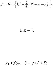
Substituting P=B into (5.6) yields

114E cannot ‘steal’ the proceeds from such liquidation, however. I also suppose that any debt payment made by E to C is verifiable.

115I rule out the possibility that C can seize E's savings. (E will have savings if B >K −w. )

It is worth going over the source of inefficiency in example 1. The assets are worth 100 in place and only 60 liquidated. Thus, in a first-best world there would be no liquidation: E would persuade C to postpone her debt and pay her 10 out of the 100 received at date 2. The trouble with such an arrangement in a second-best world is that E's promise is not credible. Whatever E may say in advance, C knows that at date 2 E will default and direct the 100 to himself. Hence C will liquidate inefficiently since it is the only way she can be repaid.

Example 2. Suppose K=90, w=30, y1=100, y2=50, L=30.

The project is obviously a profitable one (it yields 150 for an investment cost of 90) and in a firstbest world it would be financed. However, in a second-best world it will not be. The reason is that a contribution of 60 is required from C. But the most that C can recover at date 1 is 30. Moreover, even if C has all the bargaining power, E will never pay more than 50 at date 1 since the assets are worth only 50 to him at this stage. Given this, C will refuse to participate.

In example 1 inefficiency occurs because E cannot commit to hand over the second-period payoff y2 to C (in return for C agreeing not to liquidate any assets at date 1). In example 2, inefficiency occurs because E cannot commit to hand over the first-period payoff y1 to C.

3.A Multi-Period Model

There is no role for long-term debt in the above model since, given that the date 2 return, fy2, is always diverted, the date 2 debt repayment is zero. However, long-term debt becomes possible in multi-period versions of the model. This section sketches a multi-period extension; a much more detailed exposition (albeit for a slightly different model) can be found in Hart and Moore (1994a).118

118Hart and Moore (1994a) develop a dynamic theory of debt under the assumption that, rather than being able to steal the project returns, E can quit, that is, withdraw his labour from the project. E can use this threat to force C to make concessions, so that E receives a significant fraction of future cash flows from the project. (There is a close parallel between Hart and Moore (1994a) and the model used in Part I of this book, where it was also supposed that an agent could withdraw his human capital in the absence of an agreement at date 1.) The Hart–Moore (1994a) model has some advantages over the one used here. First, in many ways, the quitting assumption is more appealing than the diversion assumption. Second, the model lends itself to a continuous-time formulation and it is easy to incorporate the idea that C has some bargaining power. However, it is more difficult to include uncertainty in the model. Since I wanted to deal with the uncertainty case, at least briefly, I have chosen to work with the diversion model.

Fig. 5.2

Continue to assume perfect certainty and a zero interest rate. Consider a project that costs K and yields a return stream y1, y2, . . . , yT, as in Figure 5.2. The project can be liquidated at date t for Lt, t=1, 2, . . . , T−1, and it is worthless at date T. Write L0≡K and suppose L0≥L1≥L2≥. . .≥LT−1 (i.e. the assets depreciate). Assume also the following generalizations of (5.2)–(5.3):(5.11)

Condition (5.11) says that the project's going concern value exceeds its liquidation value at every date (including the beginning of the project).

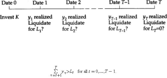
Since there is perfect certainty, one can, without loss of generality, confine attention to contracts that are never renegotiated; i.e. default never occurs.119 For simplicity, the analysis also focuses on the case where the first-best is achieved, i.e. where no liquidation occurs in equilibrium. Consider a contract that specifies the repayment path (P1, P2, . . . ,PT−1, 0). (Without loss of generality, PT can be set equal to zero, since E will divert the date T return.) Then, since E has all the bargaining power, the conditions for E not to default at dates 1, . . . ,T−1 are:

119 For a proof, see Hart and Moore (1994a). The idea is as follows. Suppose renegotiation does occur in equilibrium, at date t, say. Then at date 0 one can replace that part of the contract from date t onwards by the renegotiated contract; this yields a renegotiation-proof (or default-free) contract.

(5.12)

That is, the total debt outstanding at any time cannot exceed the liquidation value of the project.120

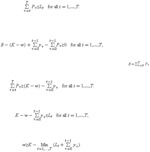
It must also be the case that E can afford to make the repayments P1, . . . ,PT1. The condition for this is(5.13)

where y0≡P0≡0. That is, the amount borrowed, net of the sum allocated towards the project, plus the total cash flows that come in from the project, must be at least as great as the cumulative debt repayments. Given (this is the break-even constraint for C), (5.13) can be rewritten as(5.14)

Combining (5.12) and (5.14) yields necessary and sufficient conditions for the first-best to be achieved,(5.15)

which can be rewritten as(5.16)

In general, there will be a continuum of repayment paths satisfying (5.12) and (5.14) (just as in the two-period model). (There is an even larger class of debt contracts sustaining these repayment paths since feasible debt contracts include those that are renegotiated on the equilibrium path, e.g. contracts consisting of large amounts of short-term debt that is rolled over.) In particular, there is a fastest repayment path, where E's outstanding indebtedness at each date (including date 0) is minimal; a slowest repayment path, where E's outstanding indebtedness at each date is

120If (5.12) does not hold, E will default and renegotiate the debt down to Lt . The formal proof of this is subtle and uses an induction argument. See Hart and Moore (1994a).

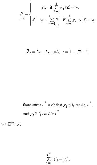
maximal; and everything in between. The fastest repayment path is given by B=K−w, and, for all t,(5.17)

That is, E borrows as little as possible and pays back as fast as possible.121 The slowest repayment path is given by =L1, and(5.18)

Here lt is the amount by which the project assets depreciate between date t and date (t+1). That is, E borrows as much as possible and pays back as slowly as possible. (E's total indebtedness is Lt at every date; recall that indebtedness cannot exceed Lt since otherwise E will default.)

The repayment paths can be used to obtain some intuition for (5.16). For simplicity, assume that, although the project returns yt can initially be less than the depreciation flows lt, once they exceed them (which they eventually must by (5.11)), they exceed them in all subsequent periods; in other words,(5.19)

Then it is easy to see that is decreasing for t≤t*+1, increasing for t≥t*+1, and reaches a minimum, M say, at t=t*+1. To understand (5.16) in this case, note that along the slowest repayment path E borrows L1 and repays at the rate of lt. Prior to date t*, E's cash flow yt falls short of lt. How does E cover the repayments? The answer is that E needs to put aside part of the initial sum borrowed in a (private) savings account, out of which he makes the shortfall lt−yt. The size of the necessary savings account is