Учебный год 22-23 / Firms, Contracts, and Financial Structure

the consequences of any action they take. (They know R(i) and C* and can figure out (4.2).) At the same time, I have supposed that transaction costs cause contractual incompleteness. There is a tension in these positions, but they are not inconsistent. There is no contradiction in assuming on the one hand that the parties cannot write a contract that specifies widget type and investment in a sufficiently unambiguous manner that a court can enforce it, but assuming on the other hand that the parties can figure out the utility consequences of their inability to write an unambiguous contract.

For example, in the house transaction described in the introduction, there are many contingencies that no contract can include. (See n. 3 of the Introduction for one of these.) But it does not follow from this that my wife and I cannot factor these contingencies into our expected utility; for instance, we might discount our utility by some amount to cover outcomes we cannot identify individually.

In reality, a great deal of contractual incompleteness is undoubtedly linked to the inability of parties not only to contract very carefully about the future, but also to think very carefully about the utility consequences of their actions. It would therefore be highly desirable to relax the assumption that parties are unboundedly rational.

Apart from making the analysis more realistic, such an approach would have other benefits too. First, it might permit the relaxation of the assumption that the parties cannot commit not to renegotiate their contract. In a world of bounded rationality, parties are unlikely to want to make such a commitment since they will wish to preserve their option to revise their contract as unanticipated events occur. Second, for similar reasons, a bounded rationality approach might allow the relaxation of the assumption that incorruptible third parties cannot be found to improve on two-party contracts. Third parties are useful to sustain message games in which M1 and M2 must pay a large penalty (to the third party) unless they agree on the appropriateness of input. However, such games will be less attractive in a world of bounded rationality where the parties may not agree either ex ante or ex post on what qualifies as ‘appropriate’ input.

It is worth noting that one can go only so far in dropping the assumption of rationality. If parties are too irrational, they may

not realize that an investment today will be expropriated by an opportunistic trading partner tomorrow. As a result, a party may invest efficiently even when it is suboptimal for him to do so; i.e. the hold-up problem may disappear! In other words, the hold-up problem—as well (probably) as the theory of asset ownership in Chapter 2—seems to rely on a minimal degree of foresight about the future utility consequences of current actions.

The Role of Asymmetric Information (Or Lack Thereof)

Asymmetric information has played a very limited role in the analysis of the hold-up problem (and plays a very limited role in the analysis in this book more generally). Variables such as R(i), C*, and i were supposed to be observable but not verifiable. I should make it clear that asymmetric information was not deemphasized because it was judged to be unimportant; rather, this was done because the analysis—particularly the analysis of renegotiation—is much more tractable under the assumption of symmetric information. Also, from a purely economic point of view it is most natural to study the hold-up problem in the context of symmetric information. The hold-up problem is most acute when M2 observes M1's investment (or observes the returns from this investment) and can exploit M1's eagerness for the widget to extract a high price. A hold-up problem can also arise if M2 is unsure about whether M1 has invested, but it is less extreme (see Tirole 1986a).

There is one place, however, where asymmetric information might be very useful. Suppose that M2's cost C* is private information. Consider a contract that states that M1 will specify a widget type (and widget price) at date 1, and M2 can either agree to M1's suggestion or decline it. In the case of symmetric information, this contract achieves the first-best if M1 has all the bargaining power. With asymmetric information, however, the first-best is not achieved since M1 may offer a price below M2's costs and M2 may decline it. But this means that M2 may pretend that her costs are high even when they are not in order to force M1 to pay more. As a result, the hold-up problem may reappear. (I say ‘may’ because, as far as I know, this case has not been analysed in the literature.) In other words, asymmetric information may help to justify the analysis of Chapter 2.

which case trade never occurs). If the bargaining game continues, then at the end of date 1 M2 makes an offer, which M1 either accepts or rejects. This ends the bargaining. There is no discounting.

Given the above timing, the following ex ante contract provides M1 with all the bargaining power. Set the no-trade price to be zero if no trade is triggered at the beginning of date 1 through M2 exercising her outside option. However, set the no-trade price to be -D, where D is a large positive number, if M2 first rejects M1's offer and then has her own offer rejected. D is essentially a large damage payment that M2 must make to M1 if bargaining continues to the end of date 1, and then breaks down.

To see why this gives M1 all the bargaining power, note that M2 will always prefer to exercise her outside option, worth zero, rather than continue with the bargaining, given the large damage payment D. It follows that M1 need only offer M2 an amount p=C* to persuade her to accept his first offer at the beginning of date 1. But this means that M1 gets all the ex post surplus; i.e. M1's payoff is(4.8)

which leads M1 to choose i=i*. That is, the first-best is achieved.

The ADR solution is ingenious, but it depends on some strong assumptions. In reality, it is hard to find anything corresponding to the outside option of no trade (for ever). Who enforces this outcome, i.e. who ensures that the bargaining game ends at this point and that M2 cannot make any further offers? Another interpretation of the ADR procedure is that, instead of there being an outside option, the damage payment is made to depend on how many offers M2 makes. That is, M2 pays no damages if she turns down M1's offer and makes no further offer, and she pays D if she does make another offer and it is turned down. However, this version supposes that, in the event of a dispute, the courts can determine how many offers M2 has made. This may not be reasonable if M2 can make secret offers. That is, having turned down M1's offer, M2 could come to M1 on the sly and propose that M1 pay her R(i) for the widget and waive the damage payment D. M1 may as well accept this offer since he will not receive D anyway. (There will be no proof that M2 made the second offer if it is rejected.) But this means that M1's net return is

(4.9)

which is maximized at i=0!

The conclusion is that the ADR procedure is likely to be valid only in particular situations. Under more general conditions, the hold-up problem reappears and the analysis of Chapter 2 becomes relevant.

2.Discussion of the Property Rights Model of Chapter 2

Given a justification for the hold-up problem, it is not difficult to provide some (tentative) support for the model of Chapter 2. Assume as in Chapter 2 that M1 requires an input from M2 and also that each party can make an investment that affects the benefits and costs of this input. (M1 chooses i and M2 chooses e.) Suppose also that the marginal returns from investment depend on how the nonhuman assets a1 and a2 are used. Moreover, there is a huge number of potential, hard-to-describe uses of these assets, only one of which, say, will be relevant in a particular state of the world. (It is supposed that each use is equally likely to be relevant.) Then a contract (of finite length) that attempts to specify particular uses will, with probability close to 1, specify only irrelevant ones, and hence what matters is who has residual rights of control—the right to choose asset uses not specified in the contract.

Given a particular ownership allocation, the parties will bargain over the gains from trade, as in Chapter 2. The logic of the present chapter can be used to show that the parties cannot gain from writing a long-term contract that specifies a no-trade price p0 and a trade price p1. The reason is that, if p1−p0 lies below the Nash bargaining price (given by (2.6)), then M2 will decline to supply and renegotiate for a higher price; while, if p1−p0 lies above the Nash bargaining price, then M1 will make an impossible demand on M2 and renegotiate for a lower price. (p0 is in effect a lump-sum transfer and has no effect on investment choice.) Thus, the only way to influence investment incentives is by allocating asset ownership.

It remains to analyse the various ownership allocations. In Chapter 2 four were discussed: M1 owns a1, M2 owns a2; M1

structures: that is, it will still be the case that, if only one party's investment matters, or only one party's investment decision is elastic, then that party should own both assets; that if assets are strictly complementary then they should be under common ownership; and that if assets are independent then they should be separately owned. Thus, while more sophisticated ownership arrangements may be an interesting embellishment to the analysis of Chapter 2, they do not undermine the message of that analysis.

3.More on the Role of the Hold-Up Problem

I have stressed that there are two crucial ingredients of the property rights approach: incomplete contracts, and residual rights of control over nonhuman assets. In the model of Chapter 2, the first ingredient was important because it led to a hold-up problem, given the non-contractibility of relationship-specific investments, while the second was important because it implied that changes in ownership could affect the severity of this hold-up problem.

It is worth pointing out that, although the hold-up problem is a useful vehicle for developing the property rights approach, it is not an essential part of the approach. That is, even in the absence of a hold-up problem, asset ownership would still generally matter. What is required for a theory of asset ownership is that there is some inefficiency in the economic relationship, which the allocation of residual control rights can influence: the inefficiency could be an ex post one rather than an ex ante one. It is worth briefly mentioning some other ways to generate inefficiency.

1.One obvious approach is to suppose that there is asymmetric information at date 1 (plus incomplete contracts at date 0). (See the discussion in Ch. 1, §3.) For example, M1 may know the value to him of the widget supplied by M2, whereas M2 may not; or M2 may know her production costs, while M1 may not. Under these conditions, ownership matters since it determines the outcome if bargaining breaks down, i.e. the parties' no-trade payoffs. Furthermore, the no-trade payoffs matter, since with positive probability bargaining will break down given the asymmetry

of information, and so the no-trade payoffs will be the actual pay-offs.

2.An even simpler—although more controversial—way to generate ex post inefficiency is to suppose that there is no (explicit) asymmetric information, but that there is a positive probability that (for unexplained reasons) M1 and M2 will simply 'not get along at date 1'. Assume that in this case the economic relationship breaks down irretrievably. (The parties no longer talk to each other and trade elsewhere.) Under these conditions, ownership again matters since it determines who can take what assets from the relationship if breakdown occurs.

3.A related approach is to suppose that the parties, rather than being opportunistic, simply have different views about the returns from various asset usages and hence disagree about how the assets should be employed; moreover, bargaining does not resolve these differences. Such an approach probably requires a departure from common knowledge, since otherwise the parties would go on talking until agreement was reached (see e.g. Aumann 1976). However, a role is again provided for asset ownership since whoever has the right to determine an asset's use will exercise this right if disagreement persists (which it will some of the time).

All these approaches seem worth exploring in future work. The end result may be a theory of integration that is richer and more realistic than the one described in Chapter 2, even if it may be 'messier' and somewhat less tractable.

Appendix

Message-Dependent Ownership Structures

In this appendix I present an example showing how a message-dependent ownership structure can be useful. For much more general discussions of the use of messages in symmetric information environments, see Maskin (1985) and Moore (1992).

To simplify, consider a case where the investment choices for M1 and M2 are discrete (invest or don't invest) and there is only one asset, a*. Treat M1 and M2 symmetrically; in particular, suppose each manager can invest 76, and each investment generates a return of 100. However, the 100 is realized only if that party has access to the asset (otherwise the investment is worthless). So if both parties invest and reach agreement about how to use the asset the gross return is 200 (and the net return is 200−152=48); while if M1 or M2 invests and can use the asset alone the gross return is 100 (and the net return is 24). In the language of Chapter 2, R=r(a*)=100, r(Ø)=0 if M1 invests; C=c(a*)=−100, c(Ø)=0 if M2 invests. (If M1 does not invest, R=r=0, and, if M2 does not invest, C=c=0.) Note that neither party needs the other party's human capital for their investment to pay off.

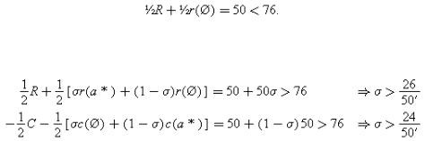
Obviously, in the first-best both parties invest. However, under a deterministic ownership structure only one party invests. Suppose M2 owns a*. Then M1 will not invest since

Similarly, if M1 owns a*, M2 will not invest. Stochastic ownership does not work any better. If M1 owns a* with probability σ and M2 with probability (1−σ), then investment by both parties requires

which cannot both be satisfied.

I now show that a combination of stochastic ownership and