SECTION 4

aliasing, but because of practical circuit limitation, the highest frequency that passes is actually about 22 kHz. Also, the anti-aliasing filter in Nyquist A/D converters requires a flat response with no phase distortion over the frequency band of interest (e.g., 20 kHz in digital audio applications). To prevent signal distortion due to aliasing, all signals above 24 kHz for a 48 kHz sampling rate must be attenuated by at least 96 dB for 16 bits of dynamic resolution.

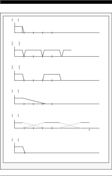
These requirements are tough to meet with an analog low-pass filter. Figure 4-1(a) shows the required analog anti-aliasing filter response, while Figure 4-1(b) shows the digital domain frequency spectrum of the signal being sampled at 48 kHz.

Now consider the same audio signal sampled at 2fs, 96 kHz. The anti-aliasing filter only needs to eliminate signals above 74 kHz, while the filter has flat response up to 22 kHz. This is a much easier filter to build because the transition band can be 52 kHz (22k to 74 kHz) to reach the -96 dB point. However, since the final sampling rate is 48 kHz, a sample rate reduction filter, commonly called a decimation filter, is required but it is implemented in the digital domain, as opposed to anti-aliasing filters which are implemented with analog circuitry. Figure 4-1(d) and Figure 4-1(e) illustrate the analog anti-aliasing filter requirement and the digital-domain frequency response, respectively. The spectrum of a required digital decimation filter is shown in Figure 4-1(f). Details of the decimation process are discussed in

SECTION 7 Digital Decimation Filtering.

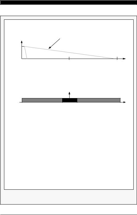
This two-times oversampling structure can be extended to N times oversampling converters. Figure 4-2(a) shows the frequency response of a general anti-alias- ing filter for N times oversamplers, while the spectra of overall quantization noise level and baseband noise level after the digital decimation filter is illustrated in Figure 4-2(b). Since a full precision quantizer was assumed, the total noise power for oversampling converters and one times Nyquist samplers are the same. However, the percentage of this noise that is in the bandwidth of interest, the baseband noise power NB is:

which is much smaller (especially when Fs is much larger than fB) than the noise power of Nyquist samplers described in Eqn. 3-4.

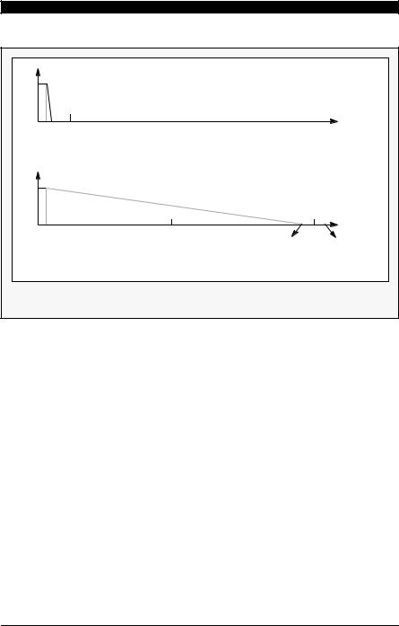
Figure 4-3 compares the requirements of the antialiasing filter of one times and N times oversampled Nyquist rate A/D converters. Sampling at the Nyquist rate mandates the use of an anti-aliasing filter with very sharp transition in order to provide adequate aliasing protection without compromising the signal bandwidth fB .

The benefit of oversampling is more than an economical anti-aliasing filter. The decimation process can be used to provide increased resolution. To see how this is possible conceptually, refer to Figure 4-4, which shows an example of 16:1 decimation process with 1-bit input samples. Although the input data resolution is only 1-bit (0 or 1), the averaging method (decimation) yields more resolution (4 bits [24 = 16]) through reducing the sampling rate by 16:1. Of course, the price to be paid is high speed sampling at the input — speed is exchanged for resolution.

Figure 4-4 Simple Example of Decimation Process

■