

text_lab1
.pdfОтчет по лабораторной работе № 1
по дисциплине «Основы анализа текстовых данных»
на тему: «Бинарная классификация фактографических данных»
Цель работы: получить практические навыки решения задачи бинарной классификации данных в среде Jupiter Notebook. Научиться загружать данные, обучать классификаторы и проводить классификацию, оценивать точность полученных моделей.
1. Импортирование необходимых для работы библиотек и модулей.
import numpy as np
from sklearn.datasets import make_classification from sklearn.metrics import confusion_matrix from sklearn.metrics import classification_report from sklearn.metrics import roc_auc_score from sklearn.metrics import accuracy_score
from sklearn.model_selection import train_test_split from sklearn.linear_model import LogisticRegression from sklearn.neighbors import KNeighborsClassifier from sklearn.ensemble import RandomForestClassifier from sklearn.naive_bayes import GaussianNB
import matplotlib.pyplot as plt
def plot_2d_separator(classifier, X, fill=False, line=True, ax=None, eps=None): if eps is None:
eps = 1.0 #X.std() / 2.
x_min, x_max = X[:, 0].min() - eps, X[:, 0].max() + eps y_min, y_max = X[:, 1].min() - eps, X[:, 1].max() + eps
xx= np.linspace(x_min, x_max, 100)
yy= np.linspace(y_min, y_max, 100) X1, X2 = np.meshgrid(xx, yy)
X_grid = np.c_[X1.ravel(), X2.ravel()] try:
decision_values = classifier.decision_function(X_grid) levels = [0]
fill_levels = [decision_values.min(), 0, decision_values.max()] except AttributeError:
# no decision_function
decision_values = classifier.predict_proba(X_grid)[:, 1] levels = [.5]
fill_levels = [0, .5, 1] if ax is None:
ax = plt.gca() if fill:
ax.contourf(X1, X2, decision_values.reshape(X1.shape), levels=fill_levels, colors=['cyan', 'pink', 'yellow'])
if line:
ax.contour(X1, X2, decision_values.reshape(X1.shape), levels=levels, colors="black") ax.set_xlim(x_min, x_max)
ax.set_ylim(y_min, y_max) ax.set_xticks(()) ax.set_yticks(())
2. Загрузка данных в соответствии с вариантом № 11.
X, y = make_classification(random_state = 15, class_sep = 0.6, n_features=2, n_redundant=0, n_informative=1, n_clusters_per_class=1,)
3. Отображение первых 15 элементов выборки:
print ("Координаты точек: ")
print (X[:15])
print ("Метки класса: ")
print (y[:15])
Координаты точек: [[-1.62644675 -0.39374849] [ 1.1229028 -0.03412507] [ 0.65583862 -0.72787224] [ 0.47374251 0.44433826] [ 1.51135743 -0.46952389] [-0.90196205 0.4449517 ] [-1.57161544 2.07402008] [ 0.79115558 0.27059781] [-0.76694954 -0.59986258] [-0.39898427 -0.34044599]
2

[ 0.33585351 -0.51983161] [ 0.68007384 1.17171521] [-0.42806409 0.41379778] [ 2.17363077 1.54353145] [ 1.42994238 1.32813118]]
Метки класса:
[0 1 1 1 0 1 1 1 0 1 0 1 1 1 1]
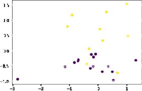
4. Отображение сгенерированной выборки на графике.
plt.scatter (X[:,0], X[:,1], c=y)
plt.show
5. Разбиение данных на обучающую и тестовую выборки в соотношении 75% - 25%.
X_train, X_test, y_train, y_test = train_test_split(X, y, test_size = 0.25, random_state = 1, )
6. Отображение на графике обучающей выборки:
plt.scatter (X_train[:,0], X_train[:,1], c=y_train) plt.show
Отображение на графике тестовой выборки: plt.scatter (X_test[:,0], X_test[:,1], c=y_test)
3
plt.show
7.Реализация моделей классификаторов, их обучение и применение на тестовом множестве.
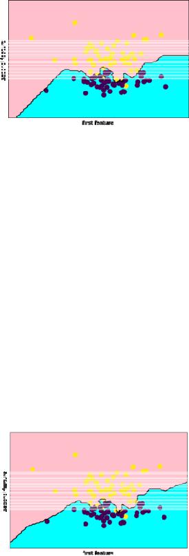
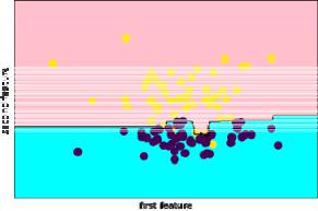
1)Метод к-ближайших соседей при n_neighbors=1:
knn = KNeighborsClassifier(n_neighbors=1, metric = 'euclidean')
knn.fit(X_train, y_train)
prediction = knn.predict(X_test)
print ('Prediction and test: ')
print (prediction)
print (y_test)
print ('Confusion matrix: ')
print (confusion_matrix(y_test, prediction))
print ('Accuracy score: ', accuracy_score(prediction, y_test))
print(classification_report(y_test, prediction))
print ('roc_auc_score: ', roc_auc_score(y_test, prediction))
plt.xlabel("first feature")
plt.ylabel("second feature")
plot_2d_separator(knn, X, fill=True)
plt.scatter(X[:, 0], X[:, 1], c=y, s=70)
Prediction and test:
[0 0 1 1 0 0 0 0 0 0 1 0 0 1 0 0 1 0 1 0 0 1 1 1 0] [0 0 1 1 0 0 0 1 0 0 1 0 0 0 1 0 1 0 1 0 1 0 1 1 0] Confusion matrix:
[[13 2] [ 3 7]]
Accuracy score: 0.8
precision recall f1-score support
4
0 |
0.81 |
0.87 |
0.84 |
15 |
1 |
0.78 |
0.70 |
0.74 |
10 |
accuracy |
|
|
0.80 |
25 |
macro avg |
0.80 |
0.78 |
0.79 |
25 |
weighted avg |
0.80 |
0.80 |
0.80 |
25 |
roc_auc_score: 0.7833333333333333
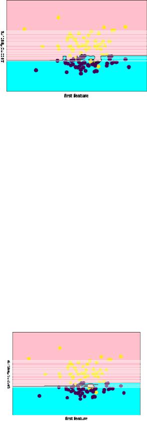
2) Метод к-ближайших соседей при n_neighbors=3:
knn = KNeighborsClassifier(n_neighbors=3, metric = 'euclidean')
Prediction and test:
[0 0 1 1 0 0 0 1 0 0 1 0 0 1 0 0 1 0 1 1 0 0 1 1 0] [0 0 1 1 0 0 0 1 0 0 1 0 0 0 1 0 1 0 1 0 1 0 1 1 0]
Confusion matrix: |
|
|
|
||
[[13 |
2] |
|
|
|
|
[ 2 |
8]] |
|
|
|
|
Accuracy score: 0.84 |
|
|
|
||
|
|
precision |
recall |
f1-score |
support |
|
0 |
0.87 |
0.87 |
0.87 |
15 |
|
1 |
0.80 |
0.80 |
0.80 |
10 |
|
accuracy |
|
|
0.84 |
25 |
|
macro avg |
0.83 |
0.83 |
0.83 |
25 |
weighted avg |
0.84 |
0.84 |
0.84 |
25 |
|
roc_auc_score: 0.8333333333333334
5
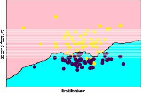
3) Метод к-ближайших соседей при n_neighbors=5:
knn = KNeighborsClassifier(n_neighbors=5, metric = 'euclidean')
Prediction and test:
[0 0 1 1 0 0 0 1 0 0 1 0 0 1 0 0 1 0 1 0 0 1 1 1 0] [0 0 1 1 0 0 0 1 0 0 1 0 0 0 1 0 1 0 1 0 1 0 1 1 0]
Confusion matrix: |
|
|
|
|
|
[[13 |
2] |
|
|
|
|
[ 2 |
8]] |
|
|
|
|
Accuracy score: 0.84 |
|
|
|
|
|
|
precision |
recall |
f1-score |
support |
|
|
0 |
0.87 |
0.87 |
0.87 |
15 |
|
1 |
0.80 |
0.80 |
0.80 |
10 |
|
accuracy |
|
|
0.84 |
25 |
|
macro avg |
0.83 |
0.83 |
0.83 |
25 |
|
weighted avg |
0.84 |
0.84 |
0.84 |
25 |
roc_auc_score: 0.8333333333333334
4) Метод к-ближайших соседей при n_neighbors=9:
knn = KNeighborsClassifier(n_neighbors=9, metric = 'euclidean')
Prediction and test:
[0 0 1 1 0 0 0 1 0 0 1 0 0 0 0 0 1 0 1 0 0 0 1 1 0] [0 0 1 1 0 0 0 1 0 0 1 0 0 0 1 0 1 0 1 0 1 0 1 1 0]
Confusion matrix: |
|
|
|
|
|
[[15 |
0] |
|
|
|
|
[ 2 |
8]] |
|
|
|
|
Accuracy score: 0.92 |
|
|
|
|
|
|
precision |
recall |
f1-score |
support |
|
|
0 |
0.88 |
1.00 |
0.94 |
15 |
6
1 |
1.00 |
0.80 |
0.89 |
10 |
accuracy |
|
|
0.92 |
25 |
macro avg |
0.94 |
0.90 |
0.91 |
25 |
weighted avg |
0.93 |
0.92 |
0.92 |
25 |
roc_auc_score: 0.9
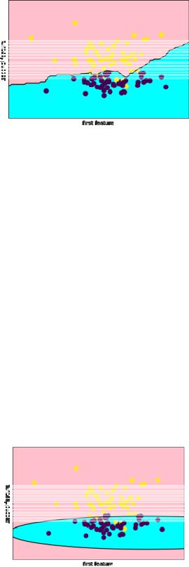
5) Наивный байесовский метод:
knn = GaussianNB()
Prediction and test:
[0 1 1 1 1 0 0 1 0 0 1 0 0 0 0 0 1 0 1 0 0 0 1 1 0] [0 0 1 1 0 0 0 1 0 0 1 0 0 0 1 0 1 0 1 0 1 0 1 1 0]
Confusion matrix: |
|
|
|
||
[[13 |
2] |
|
|
|
|
[ 2 |
8]] |
|
|
|
|
Accuracy score: |
0.84 |
|
|
|
|
|
|
precision |
recall |
f1-score |
support |
|
0 |
0.87 |
0.87 |
0.87 |
15 |
|
1 |
0.80 |
0.80 |
0.80 |
10 |
|
accuracy |
|
|
0.84 |
25 |
|
macro avg |
0.83 |
0.83 |
0.83 |
25 |
weighted avg |
0.84 |
0.84 |
0.84 |
25 |
|
roc_auc_score: 0.8333333333333334
7
6) Случайный лес при n_estimators=5:
knn = RandomForestClassifier(n_estimators=5)
Prediction and test:
[0 0 1 1 1 0 0 1 0 0 1 0 0 0 0 0 1 0 1 0 0 0 1 1 0] [0 0 1 1 0 0 0 1 0 0 1 0 0 0 1 0 1 0 1 0 1 0 1 1 0] Confusion matrix:
[[14 |
1] |
|
|
|
|
[ 2 |
8]] |
|
|
|
|
Accuracy score: 0.88 |
|
|
|
||
|
precision |
recall |
f1-score |
support |
|
|
0 |
0.88 |
0.93 |
0.90 |
15 |
|
1 |
0.89 |
0.80 |
0.84 |
10 |
|
accuracy |
|
|
0.88 |
25 |
|
macro avg |
0.88 |
0.87 |
0.87 |
25 |
weighted avg |
0.88 |
0.88 |
0.88 |
25 |
|
roc_auc_score: 0.8666666666666667
7) Случайный лес при n_estimators=10:
knn = RandomForestClassifier(n_estimators=10)
Prediction and test:
[0 0 1 1 0 0 0 1 0 0 1 0 0 1 0 0 1 0 1 0 0 1 1 1 0] [0 0 1 1 0 0 0 1 0 0 1 0 0 0 1 0 1 0 1 0 1 0 1 1 0]
Confusion matrix: |
|
|
|
||
[[13 |
2] |
|
|
|
|
[ 2 |
8]] |
|
|
|
|
Accuracy score: |
0.84 |
|
|
|
|
|
|
precision |
recall |
f1-score |
support |
|
0 |
0.87 |
0.87 |
0.87 |
15 |
|
1 |
0.80 |
0.80 |
0.80 |
10 |
8
accuracy |
|
|
0.84 |
25 |
macro avg |
0.83 |
0.83 |
0.83 |
25 |
weighted avg |
0.84 |
0.84 |
0.84 |
25 |
roc_auc_score: 0.8333333333333334
8) Случайный лес при n_estimators=15:
knn = RandomForestClassifier(n_estimators=15)
Prediction and test:
[0 0 1 1 1 0 0 1 0 0 1 0 0 1 0 0 1 0 1 0 0 1 1 1 0] [0 0 1 1 0 0 0 1 0 0 1 0 0 0 1 0 1 0 1 0 1 0 1 1 0]
Confusion matrix: |
|
|
|
||
[[12 |
3] |
|
|
|
|
[ 2 |
8]] |
|
|
|
|
Accuracy score: |
0.8 |
|
|
|
|
|
precision |
recall |
f1-score |
support |
|
|
0 |
0.86 |
0.80 |
0.83 |
15 |
|
1 |
0.73 |
0.80 |
0.76 |
10 |
|
accuracy |
|
|
0.80 |
25 |
|
macro avg |
0.79 |
0.80 |
0.79 |
25 |
weighted avg |
0.81 |
0.80 |
0.80 |
25 |
|
roc_auc_score: 0.8
9

9) Случайный лес при n_estimators=20:
knn = RandomForestClassifier(n_estimators=20)
Prediction and test:
[0 0 1 1 1 0 0 1 0 0 1 0 0 0 0 0 1 0 1 0 0 0 1 1 0] [0 0 1 1 0 0 0 1 0 0 1 0 0 0 1 0 1 0 1 0 1 0 1 1 0]
Confusion matrix: |
|
|
|
||
[[14 |
1] |
|
|
|
|
[ 2 |
8]] |
|
|
|
|
Accuracy score: 0.88 |
|
|
|
||
|
|
precision |
recall |
f1-score |
support |
|
0 |
0.88 |
0.93 |
0.90 |
15 |
|
1 |
0.89 |
0.80 |
0.84 |
10 |
|
accuracy |
|
|
0.88 |
25 |
|
macro avg |
0.88 |
0.87 |
0.87 |
25 |
weighted avg |
0.88 |
0.88 |
0.88 |
25 |
|
roc_auc_score: 0.8666666666666667
10) Случайный лес при n_estimators=50:
knn = RandomForestClassifier(n_estimators=50)
Prediction and test:
[0 0 1 1 1 0 0 1 0 0 1 0 0 1 0 0 1 0 1 0 0 0 1 1 0] [0 0 1 1 0 0 0 1 0 0 1 0 0 0 1 0 1 0 1 0 1 0 1 1 0]
Confusion matrix: |
|
|
|
|
|
[[13 |
2] |
|
|
|
|
[ 2 |
8]] |
|
|
|
|
Accuracy score: 0.84 |
|
|
|
|
|
|
precision |
recall |
f1-score |
support |
|
|
0 |
0.87 |
0.87 |
0.87 |
15 |
|
1 |
0.80 |
0.80 |
0.80 |
10 |
10