Учебное пособие 800566

где y(x) – функция формы трубы. Эта функция представляет значение амплитуды w x,t ,

–соответствующая круговая частота, i – мнимая единица. Подстановка (4) в (3) приводит к

В нем параметр имеет вид:

(2) не является точным решением (1). Следовательно, после замены (2) в (1)

получается функция ошибокR x,t :

Согласно методу Галёркина поиск неизвестных функций zi t осуществляется по условию минимизации функции ошибок R x,t в области x [0,l], где l – длина трубки.

Для этого необходимо:

После записи условия ортогональности функции ошибок всем базовым функциям получается система из n дифференциальных уравнений относительно неизвестных функций. После преобразований получается следующая матричная запись этой системы уравнений:

Для ее решения применен матричный метод. Труба разделена на участки длиной x. Учитываются следующие зависимости для функций формы:

51

Система «труба-жидкость» устойчива, если действительная часть корней характеристического уравнения отрицательна. Корни характеристического уравнения зависят от следующих величин: масс трубы и жидкости, жесткости трубы, скорости проводимой жидкости V и температуры трубы T. В зависимости от (19) может быть определена критическая скорость Vcr проводимой жидкости, при которой система теряет устойчивость.

Решение уравнения (19) представляет собой сложную задачу определения собственных значений системы даже с помощью современных компьютерных технологий и доступных программных продуктов.

Следующий подход можно использовать для определения собственных значений, что приводит к сокращению времени вычислений. Для этого система (14) преобразуется в систему дифференциальных уравнений первого порядка путем ввода новой функции q.

Корни характеристического уравнения (22) являются собственными значениями следующей задачи поиска собственных значений и собственных векторов:

В (23) c {u} обозначeн собственный вектор системы.

Эту проблему легко решить с помощью ряда математических программных продуктов.

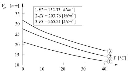
Численные исследования. Приняты следующие характеристики исследуемой системы:

E = 2.06x108kN / m2; ρf = 1000kg / m3 - объемная плотность транспортируемой жидкости; ρp = 7850kg / m3 - объемная плотность материала трубы; 10 5 oC 1

Рис. 2. Зависимость критической скорости от температуры

53

Заключение. Результаты показывают, что повышение температуры трубы T приводит к снижению критической скорости транспортируемой жидкости Vcr. Из графика рис. 2 видно, что по мере уменьшения жесткости трубы ее устойчивость также уменьшается.

Исследования показывают, что температурная нагрузка играет важную роль в устойчивости системы и должна учитываться при проектировании трубопроводов.

Библиографический список

1.Paidoussis M.P. Slender Structures and Axial Flow: Elsevier Science, 2014. – 888 p.

2.Лилкова-Маркова С., Лолов Д. Устойчивост на тръби с протичащ флуид. – София: АВС Техника, 2016. – 124 с.

3.Dynamic stability of a pipe conveying fluid with an uncertain computational model / T. Ritto, C. Soize, A. Rochinha, R. Sampaio // Journal of Fluids and Structures. – 2014. – Vol. 49. – P. 412-426 (DOI: 10.1016/j.jfluidstructs.2014.05.003).

4.Лолов Д., Лилкова-Маркова С. Расчет критической скорости флюида, протекающего в однослойной углеродной нанотрубке в полимерной матрице // Вестник ПНИПУ. Сер. Механика. – 2019. – № 4. – С.114-119.

5.Веденеев В., Порошина А.Б., Устойчивость упругой трубки, содержащей неньютоновскую жидкость и имеющей локально ослабленный участок // Труды Математического института им. В.А.Стеклова. – 2018. – № 300. – С. 42-64.

6.Qian Q., L. Wang Q., Instability of simply supported pipes conveying fluid under thermal loads // Mechanics research communications. – 2009. – Vol. 36. – № 3. – P. 413-417 (DOI: 10.1016/j.mechrescom.2008.09.011).

7.Demin Z., Baoshan L., Local Bifurcation Analysis of Parameter-Excited Resonance of Pipes under Thermal Load // Transactions of Tianjin University. – 2015. – Vol. 21. – P. 324-332 (DOI: 10.1007/s12209-015-2489-6).

8.Extremal Thermal Loading of a Bifurcation Pipe / B. Kraszewski, G. Bzymek, P. Ziółkowski, J. Badur // Scientific Session on Applied Mechanics X. AIP Conf. Proc. – 2077. – P. 020030-1–020030-9 (DOI: 10.1063/1.5091891).

9.Ameen K., Al-Dulaimi M., Hatem A., Experimental Study of Vibration on Pipe Conveying Fluid at Different End Conditions for Different Fluid Temperatures // Engineering and Technology Journal. – 2019. – Vol. 37. – Part A. N. 12 (DOI: 10.30684/etj.37.12A.3).

10.Dynamic analysis of a fluid-conveying pipe under axial tension and thermal loads / J. Gu, B. Daib, Y. Wang, M. Li, M. Duan // Ships and Offshore Structures. – 2016. – Vol. 12. – № 2. P. 1-14 (DOI: 10.1080/17445302.2015.1135564)

11.Gorman J., Sparrow W., Abraham J., Differences between measured pipe wall surface temperatures and internal fluid temperatures // Case Studies in Thermal Engineering. – 2013. – Vol. 1. – P. 13-16 (DOI: 10.1016/j.csite.2013.08.002).

12.The Influence of Fluid Temperature on the Entrance Length of Developing Flow in the Upstream Pipe of Measuring Devices / M. Alashker, M. Elrefaie, I. Shabaka, G. Mohamed // International Journal of Science and Engineering Applications. – 2019. – Vol. 8. – № 4.

– P. 124-130 (DOI: 10.7753/IJSEA0804.1004).

13.Mouloud D., Samir Z., Djilali B. Effect of Thermal Load on Vibration of ClampedClamped Pipe Carrying Fluid // Journal of Engineering and Applied Sciences. – 2020. – Vol. 15. –№ 23. – P. 3708-3712.

14.Doyle L., Weidlich I., Effects of thermal and mechanical loads on polyurethane preinsulated pipes // Fatigue and Fracture of Engineering Materials and Structures. – 2020. – Vol. 44. – № 1. – P. 1-13 (DOI: 10.1111/ffe.13347).

54

15.Fakhar M., Fakhar A., Tabatabaei H. Nanotechnology efficacy on improvement of acute velocity in fluid-conveying pipes under thermal load // International Journal of Hydromechanics. 2021. – Vol. 4. – № 2. – P. 142-154 (DOI: 10.1504/IJHM.2021.116956)

16.Investigation of temperature oscillations in a novel loop heat pipe with a vapor-driven jet injector / L. Liu, X. Yang, B. Yuan, J. Wei // International Journal of Heat and Mass Transfer. – 2021. – Vol. 179. – P. 121672.

17.Bolotin V. End deformations of flexible pipelines // Trudy Moskovskogo Energeticheskogo Instiuta. – 1956. Vol. 9. – P. 272-291.

18.Volmir S. Stability of deformable systems. – Mosсow: Nauka, 1967 – 1977.

19.Leipholz H., Stability of elastic systems // Alphen an den Rijn: Sijthoff & Noordhoff, 1980.

20.Wu S., Shih Y., Dynamic analysis of a multispan fluid-conveying pipe subjected to external load // Journal of Sound and Vibration. – 2001. – Vol. 239. – Р. 201-215.

References

1.Paidoussis M.P. Slender Structures and Axial Flow: Elsevier Science, 2014. 888 p.

2.Lilkova-Markova S., Lolov D. Stability on a test with a counter fluid. Sofia: ABC Technique, 2016. 124 p.

3.Ritto T., Soize C., Rochinha A., Sampaio R. Dynamic stability of a pipe conveying fluid with an uncertain computational model. Journal of Fluids and Structures. Vol. 49. 2014. Pp. 412-426. (DOI: 10.1016/j.jfluidstructs.2014.05.003).

4.Lolov D., Lilkova-Markova S. Calculation of the critical velocity of a fluid flowing in a single-layer carbon nanotube in a polymer matrix. Bulletin of PNRPU. Ser. Mechanics. No. 4. 2019. Pp. 114-119.

5.Vedeneev V., Poroshina A. B. Stability of an elastic tube containing a non-Newtonian fluid and having a locally weakened section. The Labors of Mathematical Institution named after V.A. Steklov. No. 300. 2018. Pp. 42-64.

6.Qian Q.L., Wang Q., Instability of simply supported pipes conveying fluid under thermal loads. Mechanics Research Communications. Vol. 36. No. 3. 2009. Pp. 413-417. (DOI: 10.1016/j.mechrescom.2008.09.011).

7.Demin Z., Baoshan L. Local Bifurcation Analysis of Parameter-Excited Resonance of Pipes under thermal load. Transactions of Tianjin University. Vol. 21. 2015. Pp. 324-332. (DOI: 10.1007/s12209-015-2489-6).

8.Kraszewski B., Bzymek G., Ziółkowski P., Badur J. Extreme Thermal Loading of a Bifurcation Pipe. Scientific Session on Applied Mechanics X. AIP Conf. Proc. 2077.-P. 020030-1–020030-9 (DOI: 10.1063/1.5091891).

9.Ameen K., Al-Dulaimi M., Hatem A. Experimental study of vibration on pipe conveying fluid at different end conditions for different fluid temperatures. Engineering and Technology Journal. Vol. 37. Part A. No. 12. 2019. (DOI: 10.30684/etj.37.12A.3).

10.Gu J., Daib B., Wang Y., Li M., Duan M. Dynamic analysis of a fluid-conveying pipe under axial tension and thermal loads. Ships and Offshore Structures. Vol. 12. No. 2. 2016. Pp. 1-14. (DOI: 10.1080/17445302.2015.1135564).

11.Gorman J., Sparrow W., Abraham J. Differences between measured pipe wall surface temperatures and internal fluid temperatures. Case Studies in Thermal Engineering. Vol. 1. 2013. Pp. 13-16. (DOI: 10.1016/j.csite.2013.08.002).

12.Alashker M., Elrefaie M., Shabaka I., Mohamed G. The influence of fluid temperature on the entrance length of developing flow in the upstream pipe of measuring devices. International Journal of Science and Engineering Applications. Vol. 8. No. 4. 2019. Pp. 124-130. (DOI: 10.7753/IJSEA0804.1004).

55

13.Mouloud D., Samir Z., Djilali B. Effect of thermal load on vibration of clamped-clamped pipe carrying fluid. Journal of Engineering and Applied Sciences. Vol. 15. No. 23. 2020. Pp. 3708-3712.

14.Doyle L., Weidlich I., Effects of thermal and mechanical loads on polyurethane preinsulated pipes. Fatigue and Fracture of Engineering Materials and Structures. Vol. 44. No. 1. 2020. Pp. 1-13. (DOI: 10.1111/ffe.13347).

15.Fakhar M., Fakhar A., Tabatabaei H. Nanotechnology efficacy on the improvement of acute velocity in fluid-conveying pipes under thermal load. International Journal of Hydromechanics. Vol. 4. No. 2. 2021. Pp. 142-154. (DOI: 10.1504/IJHM.2021.116956).

16.Liu L., Yang X., Yuan B., Wei J. Investigation of temperature oscillations in a novel loop heat pipe with a vapor-driven jet injector. International Journal of Heat and Mass Transfer. Vol. 179. 2021. P. 121672.

17.Bolotin V. End deformations of flexible pipelines. The Labors of Moscow Energetic Institute. Vol. 9. 1956. Pp. 272-291.

18.Volmir S. Stability of deformable systems. Moscow: Nauka, 1967-1977.

19.Leipholz H., Stability of elastic systems. Alphen an den Rijn: Sijthoff & Noordhoff, 1980.

20.Wu S., Shih Y., Dynamic analysis of a multi-span fluid-conveying pipe subjected to external load. Journal of Sound and Vibration. Vol. 239. 2001. Pp. 201-215.

DYNAMIC STABILITY OF A STRAIGHT PIPE CONVEYING FLUID UNDER THERMAL LOADS

D. S. Lolov1, S. V. Lilkova-Markova2

University of Architecture, Civil Engineering and Geodesy1,2

Bulgaria, Sofia

1Dr. of Technical Sciences, Associate Professor of the Department of Technical Mechanics, Tel. +359(2)9635245/767 e-mail: dlolov@yahoo.com

2Dr. of Technical Sciences, Professor of the Department of Technical Mechanics, Tel. +359(2)9635245/657 e-mail: lilkovasvetlana@gmail.com

Pipes conveying fluid are boadly used in the space industry, in nuclear reactors, in gas pipelines, in nanostructures. A number of scientists have studied the dynamic stability of such pipes from a theoretical and experimental point of view. The fluid velocities at which flutter buckling occurs are critical. The magnitude of this velocity is important in dynamic studies of fluid-conveying pipelines. This article investigates the effect of temperature load on the dynamic stability of a straight pipe conveying fluid. The static scheme of the pipe is a beam with restricted horizontal and vertical displacements at both of its ends. The velocity of the transported fluid is constant. The Galerkin method was applied for the solution of the differential equation, describing the transverse vibrations of the pipe. The characteristic equation is presented in matrix form. To solve this equation, an approach was applied that significantly reduces the calculation time. Differential equations are reduced to a first-order differential equation system. The system of differential equations is transformed and rewritten in a matrix form. It is shown that the roots of the characteristic equation are obtained by solving the generalized first order eigenvalue problem.

Results are shown for a pipe conveying fluid with specified geometric and physical characteristics. The temperature load and the critical velocity of the fluid are considered as parameters of the problem. After a numerical solution, it was found that the temperature load affects the vibrational characteristics of the pipe, as well as its critical velocity.

Keywords: stability, critical velocity, fluid, temperature load, pipe.

56

DOI 10.36622/VSTU.2022.32.1.005 УДК 624.04:531.391.3

DEFORMATIONS AND NATURAL FREQUENCY SPECTRUM OF A PLANAR REGULAR TRUSS WITH A TRIANGULAR LATTICE

M. N. Kirsanov

National Research University «MPEI»

Russia, Moscow

Doctor of Physical and Mathematical Sciences, Professor of the Department of Robotics, Mechanotronics, Dynamics and Strength of Machines, tel.: +7(495)362-73-14; e-mail: c216@ya.ru

The formula for the dependence of the deflection of a statically determined frame-type truss on the number of panels is derived by induction in the Maple computer mathematics system. A uniform and concentrated load on the upper belt is considered. A picture of the distribution of forces on the truss rods is given. The Dunkerley method is used to find a lower analytical estimate of the first oscillation frequency under the assumption that the truss mass is uniformly distributed over the nodes. Generalization of the solution to an arbitrary number of panels is carried out by induction. The solution is compared with the numerical solution for the entire frequency spectrum found using the Maple eigenvalues operator. The high accuracy of the obtained estimate is noted, which grows with the increase in the number of panels. In the set of spectra of regular trusses of various orders, spectral isolines and spectral constants are found. The error of the analytical estimate, which is a formula with coefficients in the form of polynomials in the number of panels not higher than the sixth order, does not exceed 24%. When the number of panels is more than eight, the estimation error is less than 5%.

Key words: truss, frame, Dunkerley method, oscillations, fundamental frequency, induction, isoline, Maple

Introduction

In most static calculations of building structures, numerical methods are used [1-3]. The development of methods of symbolic mathematics makes it possible to obtain analytical results as well. Such solutions are often reduced to some algorithms implemented in the systems Maple, Mathematica, Derive, Reduce, etc., but do not give compact calculation formulas [4,5]. The most difficult task is the derivation of simple calculation formulas that are valid not for anyone's construction, but a certain class. These classes include regular constructions containing periodically repeating elements in their structure. In trusses, for example, such a group can be a separate panel. The problems of the existence of statically determinate regular trusses were dealt with by Hutchinson R.G. and Fleck N.A. [6,7]. Some solutions for deflections of planar trusses of a regular type were obtained in [8-12], for spatial ones in [13]. These solutions are obtained by the inductive generalization of a series of analytical solutions with obtaining common terms of sequences of coefficients in the calculation formulas. A set of solutions for truss deflections and shifts of supports under various loads of beam, frame, arch, and cantilever trusses is contained in the reference book [14].

As a rule, in the dynamic calculations of building structures, the spectra of natural frequencies are used, and above all, the first frequency. Much less is known about analytical solutions for truss oscillation frequencies. This is primarily because the frequency equations in such problems are algebraic equations that have a high order and are not solvable in elementary functions. However, there are approximate estimates for the first frequency, which allow not only analytical solutions but also their generalizations to an arbitrary order of the regular construction [15–19]. An exact solution for the lower bound for the first frequency of a planar truss was obtained in [20].

© Kirsanov M. N., 2022

57

This paper proposes analytical solutions for planar truss deflection and first frequency estimation. The frequency spectrum of natural oscillations is investigated

Calculation of forces and deflections

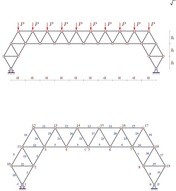
A frame-type truss (Fig. 1) has 2n panels in the crossbar and two panels each in the side parts. Truss panels are made up of equilateral triangles with side a. Truss height is 3h 3a3 / 2 . The left support of the truss is a movable hinge, the right one is fixed. The total number of bars, including the three bars modeling the supports, is 8n+22.

Fig. 1. The truss scheme n=4

Let us calculate the forces in the truss rods from the action of a uniform nodal load on the crossbar of the upper chord. All calculations and transformations will be carried out in analytical form in the Maple system according to the program [21]. We number the nodes (Fig. 2) and set their coordinates. The origin of coordinates is located in the movable support A. Here is the corresponding fragment of the program in the Maple language:

Fig. 2. Numbering of nodes and rods of the truss, n=2

for i to 3 do x[i]:=a*i/2-a/2;y[i]:=h*i-h;

x[i+2*n+2]:=a*i/2+a/2+2*n*a; y[i+2*n+2]:=3*h-h*i; end:

for i to 2*n-1 do x[i+3]:=a*i+a; y[i+3]:=2*h;

end:

58

x[i+2*n+7]:=-a/2+a*i; y[i++2*n+7]:=3*h; end:

The order of connection of rods at the nodes will be specified by special lists T[i], where i is the number of the rod, containing the numbers of the ends of the corresponding rods. For example, the lower belt is set like this:

for i to 2*n+4 do T[i]:=[i,i+1]; end:

The supports are modeled by rods of length f. Based on these data, the coefficients of the matrix of equilibrium equations of nodes in projections on the coordinate axes are calculated. Vector B on the right side of the system in odd elements contains projections of nodal loads on the x-axis, in even elements — on the vertical y-axis. In this case:

for i from 2*n+8 to 4*n+9 do B[2*i]:=-P; end;

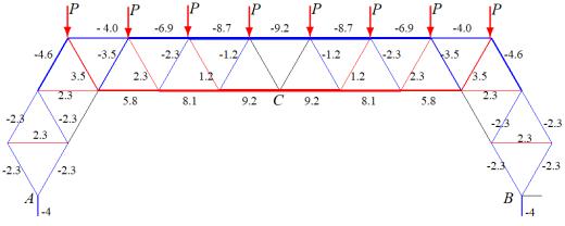
Let us present the results of the force calculation. The distribution of forces on the rods a 3m, f 1m is shown in Figure 3. Compressed rods are highlighted in blue, stretched rods are highlighted in red. The thickness of the segments of the rods is conditionally proportional to the modules of the corresponding forces. The force value is related to the value of the nodal load P and rounded up to two digits.

Fig. 3. Distribution of forces in the rods, n=3

The lower crossbar, as expected, is stretched, the upper one is compressed. The upper rods of the side parts in the lower chord are unloaded.

Deflections

Truss deflection is calculated using the Maxwell – Mohr formula

n Si(1)Si(P)li /(EF). i 1

59

Here Si(1) — is the force in the rod i from the action of a single vertical force on the node in which the deflection is measured, li — is the length of the rod i, E is the modulus of elasticity of the rods,

F is their cross-sectional area. The rigidity of the rods is assumed to be the same.

Solving the deflection problem in analytical form for n=1, 2, 3, ..., we successively obtain:

1 P(18a 2 f )/ EF,2 P(63a 3f )/ EF,3 P(172a 4 f )/ EF,

4 P(1175a /3 5f )/ EF,5 P(782a 6 f )/ EF,....

If the common term of the sequence of coefficients at f is obvious, then the common term of the sequence 18, 63, 172, 1175/3, 782 is found using the operators of the Maple system.

Thus, we have the following dependence of the deflection on the number of panels

n P((5n4 20n3 43n2 61n 33)a/9 (n 1)f )/ EF.

Similarly, we find the deflection of the truss from the action of the vertical concentrated force P at the node C

n P((8n3 24n2 49n 48)a/9 f )/(2EF).

Under the action of a vertical load, the left movable bearing receives a displacement . If in formula (1) we understand Si(1) the forces in the rods from the action of a single horizontal force on

node A, then as a result of induction on ten analytical solutions, we obtain the following value of the horizontal displacement of support A from the action of a uniform vertical load

n 2Pa3(10n3 30n2 59n 27))/ EF.

The spectrum of natural frequencies

The inertial properties of the truss are modeled by the masses concentrated in the nodes, the masses of the rods are neglected. Let us assume that the vibrations of the loads are vertical. The

accelerations of nodes with masses. The inverse of the stiffness matrix DN is the compliance matrix

BN , whose elements are calculated using the Mohr integral:

Here S(i) — is the force in the rod from the action of a unit vertical force at node i, l — is the length of the rod . Multiply (1) on the left by the matrix BN . Taking into account the

60